LLM Batching and Throughput: Why Interactive Speed Is Not the Whole System

A single fast response tells you almost nothing about whether your LLM system can handle real load. The request that feels snappy in isolation is often the same request that crawls when twenty neighbors join it—unless you understand the mechanism underneath.

The Single-Request Trap

Picture this: you've built a pipeline that summarizes support tickets. You test one ticket. The model streams back a clean summary in under two seconds. Feels great. Then you run the full backlog of five thousand tickets, and the queue crawls. Each individual call was fast. The system, as a whole, is slow.

That gap between one request feels fast and the system handles real volume is the single-request trap. It catches builders because per-request latency and system throughput are different properties, and optimizing one can hurt the other.

Latency is what one request experiences: the time from submission to completion. Throughput is the system's total output: tokens generated per second across all requests. A server can have excellent latency and terrible throughput, or excellent throughput and poor latency for any individual request.

The reason has to do with how GPUs actually serve a language model. When the GPU processes a single request, most of its time goes to moving model weights from VRAM into the compute cores—not to computing. The weights are enormous; the math per token is comparatively small. The GPU is memory-bound, meaning the memory bus is the bottleneck and the compute units sit mostly idle.

Batching changes that equation. When you process thirty requests at once, the weights still load once—but they apply to thirty different sequences of tokens. The cost of loading weights gets amortized across the whole batch, and the GPU shifts from memory-bound to compute-bound. That shift is the entire game of LLM throughput.

Why Bigger Batches Raise Throughput (and What Limits Them)

If loading weights once and applying them to many requests raises throughput, the obvious move is to make batches as large as possible. And up to a point, that works. Throughput climbs as batch size grows because each weight-loading step does more useful work.

Two constraints stop naive batching from scaling forever.

The first is memory. Every request in a batch holds a growing set of attention state called the KV cache—the keys and values the model computes for each token so it doesn't have to recompute the whole sequence at every step. That cache lives in VRAM, and it grows with every generated token. At full context length, a single request's cache can consume a gigabyte or more. The KV cache, not the model weights, is usually what caps your batch size. You run out of memory long before you run out of compute.

The second constraint is the shape of LLM generation itself. A model doesn't produce a response in one pass. It works in two phases:

• Prefill: the model processes the entire input prompt in parallel and produces the first output token.
• Decode: the model generates remaining tokens one at a time, each step depending on everything before it.

Decode is sequential and slow. And here's the problem with naive static batching: you fill a batch, run every request through prefill, then run decode until the slowest request finishes. A request that needs three more tokens waits for a batch-mate that needs three hundred. The short request sits idle, holding its KV cache in memory, while the GPU churns through tokens it doesn't care about.

This is the failure mode that makes naive batching feel broken in production. Your workload has short queries and long generations mixed together, and the short ones get dragged behind the long ones.

Continuous Batching: Filling the Gaps

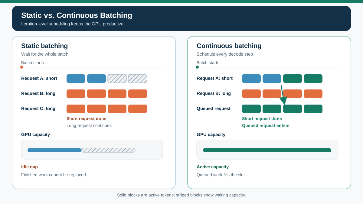
Modern serving engines solve this with continuous batching (also called iteration-level batching). Instead of scheduling whole requests, the scheduler operates at the level of individual token-generation steps.

Here's the mechanism: at each decode step, the scheduler checks which requests in the batch have finished. A finished request leaves the batch immediately—its KV cache memory is freed, and a queued request takes its place in the next iteration. The batch never waits for a straggler. The GPU stays saturated because finished requests are swapped out the moment they complete.

The latency story improves too. A short request's wait is bounded by its own tokens, not its batch-mates' tokens. That twenty-token response that would have waited a full second behind a two-hundred-token sibling now completes in roughly the time its own generation takes.

This is what powers systems like vLLM and similar modern inference engines. The throughput gains over static batching are substantial—commonly several times higher in mixed workloads, because the GPU stops idling while short requests wait on long ones.

Throughput vs. Latency: Choosing by Workload Shape

So which should you optimize? The answer depends entirely on what your workload looks like.

Offline workloads—bulk summarization, data enrichment, content generation over large datasets—should optimize throughput. Nobody is waiting on any single response. What matters is total tokens per second and cost per token. You want the largest batches your memory can hold, and you want continuous batching to keep the GPU full.

Interactive workloads—chat, search, assistants—must protect latency. Users notice time to first token, and they notice the pace of token streaming. You will deliberately run smaller batches or leave GPU capacity idle to keep interactive responses fast. That's not inefficiency; that's the price of responsiveness.

Most production systems are mixed. A chat application also runs background jobs—embedding generation, nightly summarization, log analysis. The standard pattern is a queueing layer where interactive requests jump ahead while background jobs fill whatever capacity remains. The interactive path gets its latency guarantee; the background work absorbs the leftover throughput.

The mistake I see most often is trying to maximize both metrics at once, or assuming that adding more GPUs fixes a batching problem. More GPUs add capacity, but they don't fix poor scheduling. If your batching strategy is wrong, you'll just waste more hardware.

Name your workload's dominant constraint first. Then tune batch size and scheduling around it.

Common Mistakes and How to Read the Numbers

A few errors recur across teams reasoning about LLM throughput:

Benchmarking with a single request. A one-call test tells you nothing about production behavior. It measures the best case: no queue, no contention, full memory available. Real systems degrade under load, and the shape of that degradation is what you need to know.

Treating throughput and latency as independent knobs. They are two ends of one tradeoff. Push batch size up and throughput rises while per-request latency climbs. Push latency down and you leave throughput on the table. The question is never "how do I maximize both?" It's "where does my workload need to sit on this curve?"

Ignoring workload heterogeneity. Variable prompt lengths and output lengths wreck naive batching assumptions. A dataset of long prompts with short outputs (summarization) has a completely different compute profile than short prompts with long outputs (content generation). If you benchmark with uniform requests and then run a mixed workload, your numbers will lie to you.

The metrics that matter:

• Tokens per second for throughput—measured at the batch or queue level, not the single-call level.
• Time to first token (TTFT) for interactive paths. This is what users perceive as "the model starting to respond."
• Time per output token (TPOT) for streaming feel. Users notice when tokens arrive slowly.

Measure at the batch or queue level before you judge a serving setup. A single fast call is a demo. A queue that drains predictably under mixed load is a system.

The Decision Rule

Here's where I'd start if you're building on top of an LLM serving stack:

1. Name your workload's dominant shape. Interactive, offline, or mixed?
2. Pick the governing metric. For interactive, it's TTFT and TPOT. For offline, it's tokens per second and cost per token. For mixed, design the queueing layer first.
3. Run one load test that measures throughput and latency together. Send a realistic mix of request lengths and arrival patterns. Watch what happens to the queue as concurrency rises.

Interactive speed is a feature of one request. Throughput is a property of the whole system. Builders who confuse the two optimize the wrong number—and end up with a demo that feels fast and a production system that crawls.

References

Research updated Sep 7, 2026