
LLM Batching and Throughput: Work Through the Numbers
Throughput climbs, the dashboard looks healthy, and p95 quietly doubles. Here is the arithmetic that explains why.

Key topics
Throughput climbs, the dashboard looks healthy, and p95 quietly doubles. Here is the arithmetic that explains why.
A serving dashboard shows throughput rising as you raise the batch limit. Someone on the team pushes it higher, the chart looks better, and the average latency barely moves. Then a user complains that answers feel slow, and the p95 wait time has quietly doubled. Nothing broke. The system did exactly what the configuration asked for. The problem is that "bigger batch equals better system" is not a model. It is a slogan, and it cannot tell you when to stop.
So let's replace it with something you can compute on the back of an envelope. By the end of this article you will be able to estimate requests-per-second throughput and per-request waiting from two numbers: batch size and service time. No vendor benchmark required.
If you already understand that latency and throughput are different quantities, this article only adds arithmetic to that distinction. If that distinction is still fuzzy, the short version is enough to continue: latency is what one request experiences, throughput is what the system completes per unit time, and they can move in opposite directions.
The Two Numbers You Are Actually Trading
Fix the notation first, because every later example depends on it.
- Service time (S): the time to process one batch end to end, from the moment the batch starts until its last token is produced.
- Batch size (B): the number of requests processed together in that batch.
- Throughput: requests completed per unit time.
- Waiting (W): the time a request spends queued before its batch begins.
The core identity is almost embarrassingly simple:
Read it as a sentence. Throughput improves only when B grows faster than S. If you double the batch size and service time also doubles, you have bought nothing. If you double the batch size and service time grows by 20 percent, you have bought a lot. The entire trade lives in the ratio.
This model assumes uniform request lengths, a single worker, and static batching — requests are grouped, processed together, and the batch is not refilled until it finishes. Each assumption matters. Variable output lengths mean the batch runs until its longest member finishes, so short requests pay for long ones. Multiple workers change the arithmetic but not the shape. Continuous batching, where new requests join mid-flight, breaks the model in a useful direction, and we will come back to that boundary.
Knowledge check
Check your understanding
Answer this question before you continue.
Why Service Time Does Not Scale Linearly With Batch Size
If throughput were simply B divided by S, and S stayed constant, throughput would grow forever with batch size. It does not. So the real question is: what does S actually do as B grows?
Split a batch into two phases. Prompt processing reads the input tokens and builds the KV cache. This phase parallelizes well across requests, because the work is mostly matrix multiplication over many tokens at once. Decoding generates output tokens one step at a time, and each step must read the model weights plus the KV cache for every active sequence from memory. That read is the bottleneck, not the arithmetic.
Here is the argument in plain steps:
- At batch size 1, a decode step reads the full model weights to produce a single token. The compute units sit mostly idle while memory moves data.
- At batch size 8, the same weight read produces 8 tokens. The marginal cost of those extra 7 requests is small — mostly KV cache reads.
- At batch size 64, the KV cache itself is large. Now the read includes weights plus a substantial cache, and the marginal cost per added request grows.
- At very large batches, the cache dominates memory traffic, and each added request costs nearly as much as the first.
The consequence is that S(B) is sublinear at small B and approaches linear at large B. Throughput, B divided by S, therefore rises steeply at first and then flattens. The batch size where the flattening becomes pronounced is the saturation point: the point where added requests stop buying throughput and start buying only waiting.
Warning: Past saturation, larger batches can reduce throughput, not just flatten it. Memory pressure, KV cache eviction, or an outright out-of-memory error will cost you more than the batch gained.
Knowledge check
Check your understanding
Answer this question before you continue.
Worked Example: Throughput at Three Batch Sizes
Let's put numbers on it. Suppose one worker, a fixed output length, and three candidate batch sizes. The service times below are illustrative arithmetic, chosen to show the shape — not a benchmark from any specific model or GPU.
| Batch size (B) | Service time (S) | Throughput (B/S) | Marginal gain |
|---|---|---|---|
| 1 | 1.0 s | 1.00 req/s | — |
| 4 | 1.6 s | 2.50 req/s | +1.50 req/s |
| 16 | 4.0 s | 4.00 req/s | +1.50 req/s |
| 64 | 14.0 s | 4.57 req/s | +0.57 req/s |
Look at the marginal column. Going from 1 to 4 buys 1.5 requests per second. Going from 4 to 16 buys another 1.5. Going from 16 to 64 buys 0.57. The curve is flattening, and the flattening is visible in the arithmetic, not asserted by a chart.
Now translate the table back into behavior. The jump from 16 to 64 raises throughput by about 14 percent, but it raises service time from 4 seconds to 14 seconds. Every request in that batch now occupies the worker for three and a half times as long. If your workload is interactive, you just paid a large latency bill for a small throughput gain.
Note: These constants depend on the model, the hardware, the sequence length, and the serving engine. The shape is general; the numbers are not. Measure your own.
Knowledge check
Check your understanding
Answer this question before you continue.
Where Waiting Comes From
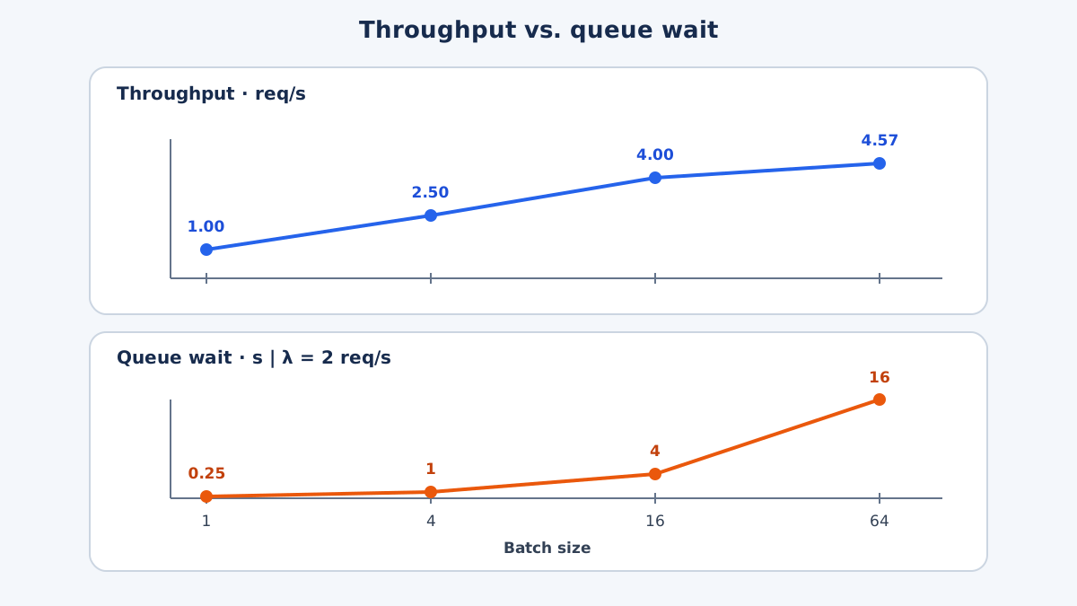
Throughput is only half the trade. The other half is the time a request spends waiting for its batch to fill.
Let λ (lambda) be the arrival rate in requests per second. A request that arrives when the batch is empty must wait for enough companions to justify starting. On average, a request arrives halfway through the fill window, so:
The total time a request spends in the system is waiting plus service:
Notice the asymmetry that matters. Throughput is a system property; waiting is a per-request property. A batch size that looks excellent on a throughput chart can be miserable for a single user, because the user experiences the wait, not the aggregate.
Run a quick case. At λ = 2 requests per second and B = 16, the average wait is 16 divided by 4, or 4 seconds — before service even starts. At B = 4, the wait drops to 1 second. The throughput difference between those two configurations, from the table above, is 1.5 requests per second. Whether that is worth 3 extra seconds of waiting is a workload question, not a math question.
Common mistake: At low arrival rates, a large batch size means requests sit in the queue waiting for company that may never arrive. If λ is small, the fill time dominates and the worker idles either way. A smaller batch — or no batching — often wins outright.
Knowledge check
Check your understanding
Answer this question before you continue.
Interactive Versus Offline: Same Formula, Different Constraint
The formulas do not change between workload shapes. What changes is which constraint binds.
Interactive workloads bind on waiting. A human is watching the response. The batch size is capped by the maximum acceptable queue delay, and throughput is whatever falls out of that cap. You do not choose throughput; you choose a latency budget and accept the throughput it permits.
Offline workloads bind on throughput. No human is watching. Waiting is nearly free, so push batch size toward the saturation point and accept long per-request times. A document-processing job that finishes in an hour instead of three is a win even if each individual document takes longer.
| Interactive | Offline | |
|---|---|---|
| Binding constraint | Waiting (W) | Throughput (B/S) |
| What you maximize | Responsiveness | Requests per unit time |
| What you tolerate | Lower throughput | Long per-request time |
| Typical mistake | Raising batch size to chase the throughput chart | Capping batch size out of latency habit |
The boundary where this model stops being exact is worth naming. Variable output lengths mean a batch runs until its longest member finishes, so the effective service time is set by the maximum, not the average. Continuous batching changes the arithmetic further by letting new requests join mid-flight, which is why real serving systems often beat the static model's predictions. Once you understand the static case, measuring the dynamic case is the natural next step.
Choosing a Batch Size Without Guessing
Here is the procedure I would run on any new workload.
Step one: measure service time at two or three batch sizes. Use your own model and hardware. A published table from different hardware will mislead you, because the constants depend on memory bandwidth, model size, and sequence length.
Step two: compute throughput and average waiting for each. Use B/S for throughput and B/(2λ) for waiting. Find the batch size where the marginal throughput gain drops below what the added waiting costs you.
Step three: set the cap from your binding constraint. Interactive: cap by the maximum acceptable queue delay. Offline: cap near the saturation point.
Three mistakes to check for before you ship a config:
- Tuning batch size before fixing output length variance. High variance wastes batch slots and distorts every measurement.
- Reading average latency while p95 degrades. Averages hide the tail, and the tail is what users complain about.
- Assuming a benchmark from different hardware transfers. It does not.
Tip: Pick the smallest batch size that reaches your throughput target. Everything above it is waiting you did not need to buy.
The immediate next action is to measure service time on your own workload at two batch sizes and compute the ratio. That single measurement will tell you more than any published benchmark. Once the static model is clear, the natural next topic is continuous batching and how variable output lengths change the arithmetic — because that is where the hand-computable model meets the systems that actually serve production traffic.
Knowledge check
Final check
Finish the article by checking the ideas you just learned.
References
Want a more structured LLMOps path?
Use the LLMOps Practical Starter Bundle to connect RAG, evaluation, observability, and production patterns.
Large Language Models Starter Pack
A 12-chapter guide connecting LLM fundamentals with prompting, RAG, agents, tool calling, evaluation, security, and application engineering.
- 227-page Illustrated PDF edition
- 12 guided LLM engineering chapters
- Visual concept diagrams
- Self-assessment quizzes
- Bonus deep-dive sections
- Prompt design, structured output, context windows & RAG pipelines
- Agents, tool calling, prompt injection, evaluation & application lifecycles
Coming soon


