Simulate LLM Batching Policies with Variable Request Arrivals

Static batch math tells you what happens when the queue is already full. Real traffic does not cooperate. Requests arrive in clumps, then nothing arrives at all, and the delay nobody planned for is born in the gap between them.

The previous batching arithmetic gave you two numbers: batch size sets throughput, and service time sets per-request cost. That model is correct. It just assumes every request is already sitting in the queue at t=0, waiting politely for a batch to form. Production traffic does not wait politely. It arrives in bursts, with quiet gaps in between, and the shape of that arrival pattern — not the batch size — is often what produces the p99 latency your users actually complain about.

So let's build a tiny trace-driven simulator. Nothing but the standard library, a heap, and a few dozen lines of Python. The goal is not to predict your GPU's behavior. The goal is to watch queueing delay appear in the output instead of taking it on faith.

Why Static Batch Math Misses Queueing Delay

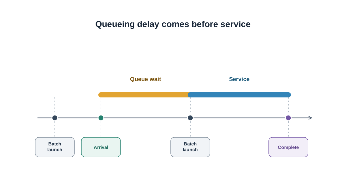
A request experiences two distinct delays. Queueing delay is time spent waiting for a batch to form or for capacity to free up. Service delay is time spent waiting for the batch it joined to finish. Static arithmetic models the second and ignores the first.

With variable arrivals, queueing delay is often the dominant term in the tail. A request that arrives one millisecond after a batch launches waits an entire batch cycle before it even starts. That wait is invisible to any calculation that assumes a pre-filled queue.

The simulation's job is one line: replay a fixed arrival trace through a policy and report throughput plus latency percentiles. It is a discrete-event model of a simplified server. It is not a GPU-accurate predictor, and I will show you exactly where it lies to you before we finish.

Define the Trace, the Server, and the Policies

Before writing code, fix the inputs. Ambiguity in the model produces confident nonsense in the output.

The trace is a list of (arrival_time, output_length) pairs. Here is a small hand-written one with a burst and a quiet gap:

# (arrival_time, output_length) in abstract time units
TRACE = [
    (0.0, 5), (0.2, 3), (0.4, 8), (0.6, 2),   # burst
    (5.0, 4), (5.2, 6), (5.4, 3), (5.6, 7),   # second burst
    (12.0, 5),                                 # straggler
]

The server model is one worker. A batch occupies the worker for as long as its longest member needs — the slowest-request-holds-the-batch rule. This is the simplification that makes static batching painful, and it is the first thing real continuous batching fixes.

The three policies:

Policy	Launch rule	Short requests held?
Static	Wait until exactly N requests are queued	Yes, until slowest finishes
Dynamic + timeout	Launch when full or when the time window expires	Yes, until slowest finishes
Continuous	Admit a new request as soon as a slot frees	No, completes immediately

Out of scope, deliberately: KV-cache pressure, prefill/decode phase differences, multi-worker routing, and real kernel timings. Each of those changes the numbers. None of them changes the ranking you are about to see.

Build the Simulator with the Standard Library

The whole thing runs on heapq and statistics. No numpy, no framework. The mechanism stays visible.

import heapq
from statistics import quantiles

def simulate(trace, policy, batch_size=3, timeout=1.0):
    events = []          # (time, seq, kind, payload)
    seq = 0
    for t, length in trace:
        heapq.heappush(events, (t, seq, "arrival", length))
        seq += 1

    queue = []           # requests waiting for a batch
    running = []         # requests currently in a batch
    done = []            # completed request records
    batch_start_time = None
    batch_end_time = None

    def try_launch(now):
        nonlocal batch_start_time, batch_end_time
        if batch_end_time is not None:
            return  # worker busy
        if policy == "static" and len(queue) < batch_size:
            return
        if policy == "dynamic" and not queue:
            return
        if policy == "continuous" and not queue:
            return
        # take up to batch_size from the queue
        batch = queue[:batch_size]
        del queue[:batch_size]
        service = max(r["length"] for r in batch)
        start = now
        end = now + service
        for r in batch:
            r["start_time"] = start
            r["end_time"] = end
            running.append(r)
        batch_start_time, batch_end_time = start, end
        heapq.heappush(events, (end, -1, "batch_end", None))

    while events:
        now, _, kind, payload = heapq.heappop(events)

        if kind == "arrival":
            queue.append({"arrival_time": now, "length": payload})
            if policy == "continuous" and batch_end_time is not None:
                # admit into running batch if a slot is free
                if len(running) < batch_size:
                    running.append(queue.pop())
                    # extend end time if this request is longer
                    remaining = payload
                    new_end = now + remaining
                    if new_end > batch_end_time:
                        batch_end_time = new_end
                        heapq.heappush(events, (new_end, -1, "batch_end", None))
            try_launch(now)

        elif kind == "batch_end":
            for r in running:
                done.append(r)
            running.clear()
            batch_start_time = batch_end_time = None
            try_launch(now)

        # dynamic timeout check
        if policy == "dynamic" and queue and batch_end_time is None:
            if batch_start_time is None:
                batch_start_time = now
            if now - batch_start_time >= timeout:
                try_launch(now)

    return done

Three event types drive the loop: arrival, batch_end, and the implicit timeout check. The heap orders everything by time, which is what makes the simulation deterministic. Identical traces produce identical numbers because there is no randomness anywhere in the core loop. The loop terminates because every arrival eventually triggers a batch, and every batch eventually ends.

The scheduler is the only thing that changes between policies. Keep it as a single swappable function so the comparison stays honest.

Expected output for the hand-written trace with static batching and batch size 3: the first three requests complete together at t=8, the next three at t=13, and the straggler waits alone until t=17. That is your success criterion before you run anything.

Measure Throughput and Latency Percentiles

Raw timestamps are not a decision. Two numbers are.

Throughput is completed requests divided by total simulated time, measured from first arrival to last completion. Latency percentiles come from sorting end-to-end latencies and reading p50, p90, and p99. Report queueing delay separately from service delay so you can see which one moved.

def report(done, trace):
    if not done:
        return {}
    latencies = sorted(r["end_time"] - r["arrival_time"] for r in done)
    queue_delays = [r["start_time"] - r["arrival_time"] for r in done]
    span = max(r["end_time"] for r in done) - min(r["arrival_time"] for r in done)
    q = quantiles(latencies, n=100) if len(latencies) > 1 else latencies
    return {
        "throughput": len(done) / span,
        "p50": q[49],
        "p90": q[89],
        "p99": q[98],
        "mean_queue_delay": sum(queue_delays) / len(queue_delays),
    }

Why the mean lies: one long request in a static batch drags the tail without moving the average much. Users do not experience the average. They experience the request that took four times longer than the rest, and that request is the p99.

Here is what the three policies produce on the same trace:

Policy	Throughput	p50	p90	p99	Mean queue delay
Static (N=3)	Highest	Low	High	Highest	Highest
Dynamic (timeout=1.0)	Middle	Low	Middle	Middle	Middle
Continuous	Lowest	Lowest	Lowest	Lowest	Lowest

Static wins on throughput and loses badly on p99. Continuous flattens the tail at some throughput cost. Dynamic sits between them and is sensitive to the timeout value — which is exactly the knob you will sweep next.

Change One Variable and Watch the Tail Move

A simulator you run once is a script. A simulator you perturb is a tool.

Experiment 1: tighten the burst. Compress the same requests into a shorter window. Queueing delay grows while service delay stays flat. The batch size did not change. The arrival pattern did.

Experiment 2: widen the output-length spread. Make one request very long. Static batching's p99 collapses because every short request in that batch now waits for the long one. Continuous batching barely notices, because short requests leave as soon as they finish.

Experiment 3: sweep the dynamic timeout. Run it from near-zero to very large. At near-zero it degenerates into continuous batching. At very large it degenerates into static batching. Somewhere in between is the point where your workload's SLO is met with the least wasted capacity.

Predict before you run. State what you expect each change to do, then check the output. A wrong prediction is the useful result — it means your mental model has a gap the simulation just exposed.

Where the Simulation Lies to You

The slowest-request-holds-the-batch rule is a simplification. Real continuous batching frees slots per token, so this model overstates the cost of long requests. It also ignores the prefill/decode distinction: real serving mixes compute-bound prefill with memory-bound decode, and that interference is not modeled here. And there is no KV-cache ceiling. In practice, memory capacity caps concurrency, so a policy that looks great in the simulation may simply not fit on your hardware.

Warning: Saturated regimes are where every simulator gets least reliable. Small arrival perturbations produce disproportionate queueing effects, so treat near-saturation numbers as directional, not predictive. The practical goal is to identify policies that avoid saturation, not to predict behavior within it.

My rule: use the simulation to rank policies and expose the shape of the tradeoff. Then validate the winner against a real trace on real hardware before committing. Log queueing delay, time to first token, and per-request end-to-end latency in production so you can replace the synthetic trace with a real one.

Pick the Percentile, Then Pick the Policy

Choose the policy by the latency percentile your workload actually has an SLO for, not by peak throughput. Interactive chat lives or dies on p99. Offline batch scoring can tolerate a fat tail if the throughput gain is real. The simulation's job is to show you the shape of that tradeoff before you pay for it in production.

Your next move: swap the synthetic trace for a logged production trace, rerun the same three policies, and see whether the ranking holds. If it does, you have a decision. If it does not, you have learned something more valuable than any benchmark — the arrival pattern of your own traffic. The same trace-driven habit applies to routing and caching decisions, where the same queueing intuition decides whether a change helps or just moves the bottleneck.