Inference-Time Compute: Reasoning About Extra Model Effort

A builder doubles the candidate count, watches the benchmark number climb, ships it, and then discovers that p95 latency and per-request cost moved in ways nobody modeled. The quality gain was real. The bill was also real, and it arrived on a different schedule.

That gap between "quality went up" and "the spend was justified" is where most inference-time compute decisions go wrong. The fix is not a better rule of thumb. It is an explicit model you can plug numbers into before you commit a workflow to production.

This article builds that model. We will define two bounded workflows precisely, state the notation, derive cost and latency, run one worked example, and then draw a hard line between what the arithmetic proves and what only measurement can tell you.

Two Bounded Workflows, Defined Precisely

Extra inference-time compute is not a quality dial. It is a budget allocation, and it only converts into quality when something downstream can tell a better answer from a worse one.

The comparison in this article is between exactly two workflows. Naming them precisely is what makes the arithmetic mean anything.

Workflow A — single-pass generation. One decode, one answer. Nothing selects, nothing compares. Cost and latency scale with output length.

Workflow B — parallel candidate generation plus one verification pass. The model samples N candidates concurrently. A separate verification pass then scores the candidate set and returns the best one. The verifier does not generate new answers; it only ranks what it was given.

That is the whole model. It is deliberately narrow. If you want to compare majority voting against best-of-N ranking, or a verifier that repairs candidates instead of selecting them, those are different workflows with different cost and latency shapes — and you should model them separately rather than smuggling them into one equation.

The load-bearing distinction: candidate generation expands the space of answers; verification selects within it. Sampling without a usable selector is noise with a bill. You paid for four answers and shipped the same distribution you started with.

Note: Published results on inference-time scaling show gains that saturate, and in some settings fail to materialize entirely. Treat "more compute helps" as a hypothesis about your task, not a law about models.

If you already understand how token volume drives cost and latency at the request level, that background carries forward here. What changes is that we are now making the allocation decision explicit rather than re-deriving the basics.

Notation and Assumptions

Before any arithmetic, name every symbol. The model is only as honest as its assumptions.

Let:

• c = cost per candidate (one full generation)
• v = cost of the verification pass over the candidate set
• N = number of candidates sampled in parallel
• L₁ = latency of a single-pass generation
• ΔL = marginal wall-clock latency added by each additional parallel candidate
• ΔV = wall-clock latency added by the verification pass
• q(N) = probability the selected answer is correct, given N candidates and one verification pass

That last term is the one that matters and the one the model cannot supply. Quality is a task-specific success probability, not a vague "better." You measure it; the model does not predict it.

The budget is a constraint pair, not a single number: a latency ceiling and a cost ceiling per request. Both must hold. A strategy that clears cost but blows latency is not a candidate.

Three assumptions hold the model together, and each one can break:

1. Candidates are drawn from a fixed model. Swapping models mid-experiment invalidates the comparison.
2. Verification is imperfect. The verifier has its own error rate.
3. Quality is monotone only up to a saturation point. Past that knee, more candidates buy nothing.

The assumption that breaks most often is subtler: verification quality is independent of candidate quality. When the verifier shares the generator's blind spots, extra candidates raise confidence without raising correctness. The system agrees with itself, loudly, and is wrong in the same direction every time.

Modeling the Tradeoff

Now derive the two expressions step by step.

Total cost is the sum of generation and verification spend:

Each candidate costs c; the single verification pass costs v. Cost scales linearly in N.

Total latency starts from the single-pass baseline and adds the marginal cost of each extra candidate and the verification pass:

The (N − 1) term is there because the first candidate is the baseline. Everything after it is added work. The ΔL term assumes candidates run concurrently, so each additional candidate adds a bounded marginal delay rather than a full generation's worth of time. If your runtime serializes candidates, replace (N − 1) · ΔL with (N − 1) · L₁ — the arithmetic changes, and so does whether the workflow fits an interactive ceiling.

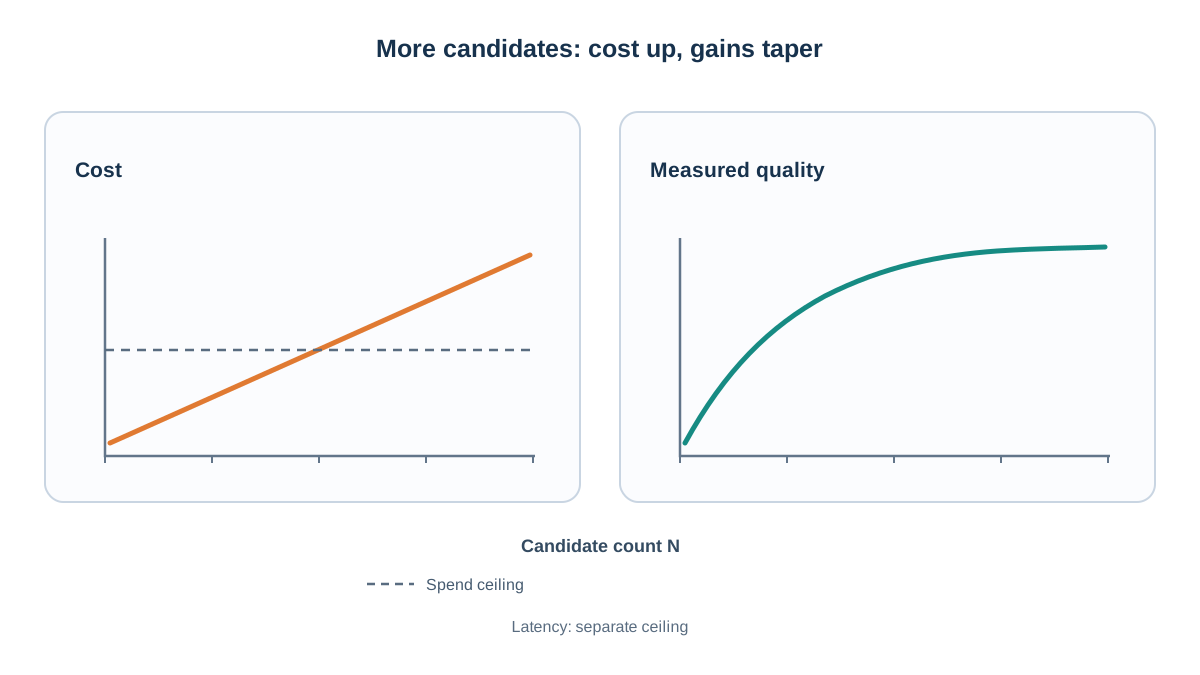
Here is the whole story in one mismatch: cost scales linearly in N, while quality typically scales sublinearly and saturates. Double the candidates and you roughly double the cost. You do not roughly double the quality. You get a shrinking increment, and eventually none.

That mismatch turns the decision into a marginal question: does the next candidate buy more expected quality than it costs in budget? The model cannot answer that for you. It can only tell you what quality you would need for the spend to be justified. That is a different and more useful thing.

Picture two axes: budget on one, quality on the other. The quality curve rises, bends, and flattens at a saturation knee. The budget line rises straight and never bends. The point where the flat curve stops outrunning the straight line is where extra candidates stop paying.

A Worked Example

Pick a concrete shape: a structured extraction task with a stated latency ceiling of 2,000 ms and a cost ceiling of $0.02 per request.

Assume these numbers:

• c = $0.002 per candidate
• v = $0.003 per verification pass
• L₁ = 400 ms
• ΔL = 150 ms
• ΔV = 300 ms

Option A — single pass. Cost = $0.002. Latency = 400 ms. Both ceilings clear easily.

Option B — N = 4 with verification. Cost = 4 × $0.002 + $0.003 = $0.011. Latency = 400 + 3 × 150 + 300 = 1,150 ms. Both ceilings clear.

Now push N. At N = 8, cost = 8 × $0.002 + $0.003 = $0.019 and latency = 400 + 7 × 150 + 300 = 1,750 ms. Cost is approaching the ceiling; latency is still fine. At N = 10, cost = $0.023 — over the ceiling — while latency = 2,050 ms, also over. Cost breaks first, but only just.

Notice what just happened. The cost and latency numbers are arithmetic consequences of the model. They are not opinions. The quality numbers are not in this calculation at all, because they cannot be.

So run the sensitivity check. Suppose a held-out evaluation on your task gives Option A a quality of 0.70 and Option B at N = 4 a quality of 0.82. Option B is worth its extra $0.009 and 750 ms. Now suppose the same evaluation shows the verifier is only marginally better than chance at ranking candidates on this task — say it picks the correct candidate 55% of the time when the correct one is present. Option B's measured quality drops toward Option A's while its cost and latency stay fixed. The ranking flips. Nothing about the arithmetic changed. Only a measured input did.

Common mistake: Treating the quality column as if it came from the same source as the cost column. Cost is derived. Quality is assumed until you measure it on your own task.

When Extra Effort Pays Off — and When It Does Not

Turn the model into decision boundaries.

Use extra effort when: the task has a checkable success criterion, errors are costly, the latency budget is generous, and the verifier is genuinely independent of the generator.

Skip it when: the task is latency-critical, the answer is not verifiable, or the failure mode is a confident wrong answer that a weak verifier will happily approve.

Three failure modes deserve names.

Verification theater. A second pass that agrees with the first because it shares the same context and the same blind spot. You paid for two opinions and got one, echoed.

Budget creep. N grows because N is easy to change, while nobody re-measures whether quality moved. The knob turns; the needle does not.

Adversarial and open-ended settings. In these, additional compute has been observed to help less, or not at all, and can even be steered unproductively. More thinking is not automatically better thinking.

The decision rule: choose the smallest N that clears your quality threshold under both ceilings, then stop. Re-check the threshold when the task or the model changes, because the saturation knee moves with them.

What the Model Does Not Prove

Close the loop on the split that has run through this whole article.

Cost and latency conclusions follow from arithmetic. If your per-candidate cost and marginal latency are right, the totals are right.

Quality conclusions follow only from measurement on your own task. Three specific claims are assumption-dependent, and you should treat each as unproven until you test it:

• That verification is independent of generation.
• That quality saturates rather than degrades as N grows.
• That the verifier's errors are uncorrelated with the generator's.

None of these are guaranteed. All of them are checkable.

The next move is small and concrete. Instrument one real task. Record single-pass quality, then N = 2 and N = 4 with a verifier. Plot quality against cost and latency before you change anything in production. The model becomes a tool you test rather than a belief you adopt — and the moment you have that plot, you will know which of your assumptions was doing the real work.