
LLM KV Cache Memory: Work Through the Inference Math
The weights fit. The model loads. Then the second concurrent request arrives, and the server refuses to admit it.

Key topics
The weights fit. The model loads. Then the second concurrent request arrives, and the server refuses to admit it.
Nothing about the model changed between the first request and the second. What changed is that the first request is still holding per-token state in device memory, and that state grows with every token it generates. The KV cache is not a speed trick that happens to cost a little memory. It is per-request state that scales with tokens times concurrency, and it competes with the weights for the same pool of GPU memory.
By the end of this article you will be able to estimate that number on paper — before you rent the GPU.
What the Cache Actually Stores
During prefill, the model processes the whole prompt and computes a key vector and a value vector for every token, at every layer. During decode, it computes K and V for exactly one new token per layer per step, appends them, and reuses everything already stored. That reuse is what turns per-step attention cost from recomputing the entire prefix into reading stored state.
The compute saving is real. So is the memory bill.
Three properties matter for the arithmetic:
- Each layer keeps its own K and V. The cache is not one shared tensor; it is L separate pairs of tensors, one pair per layer.
- The cache is per-request. Model weights are fixed and shared across every request the server handles. The KV cache is created when a sequence starts, grows token by token, and is discarded when the sequence ends.
- The cache is not an answer cache. A response or semantic cache stores finished outputs keyed by request similarity. The KV cache stores internal attention state for one in-flight sequence. Same word, different object, different failure modes.
Common mistake: Treating the KV cache as a speed optimization that is "basically free." It is free only while sequences are short and concurrency is low. Past that boundary, it is the constraint.
Knowledge check
Check your understanding
Answer this question before you continue.
Notation and Assumptions
Before deriving anything, name the symbols:
| Symbol | Meaning |
|---|---|
| Number of transformer layers | |
| Cached tokens for one sequence (prompt plus generated) | |
| Concurrent sequences (batch size) | |
| Number of key-value heads | |
| Head dimension | |
| bytes | Bytes per stored element (2 for FP16/BF16, 4 for FP32) |
deserves its own line. In multi-head attention, every attention head has its own K and V, so equals the total head count. In grouped-query attention, several query heads share one K/V head, which cuts while leaving the query head count untouched. That single architectural choice is the largest lever on cache size, and it is why the formula cannot always be collapsed into a model-dimension shortcut.
The simplifying assumptions, stated up front:
- Uniform layer shape — every layer has the same and .
- No sliding-window or sparse attention — every cached token stays resident.
- No cache quantization — one dtype throughout.
- No prefix sharing between requests.
- The cache lives entirely in device memory.
- counts the full cached length, prompt included.
Real serving stacks add allocator overhead, fragmentation, and padding, which push actual allocation above this estimate. Prefix sharing and eviction can push it below. Treat the result as a baseline under the listed assumptions, not a measurement.
Knowledge check
Check your understanding
Answer this question before you continue.
Deriving the Per-Token Cost
Build the formula one factor at a time.
One token, one layer. The layer stores one key vector and one value vector, each of size elements. That is elements per token per layer.
All layers. Each layer keeps its own copy, so multiply by :
Bytes. Multiply by the dtype width:
The multi-head simplification. When equals the full head count, the product equals the model dimension , because the heads together span the full representation space. The formula collapses to per token. This is the form you will see quoted most often.
Where the shortcut breaks. Under grouped-query attention, , so . Substituting here overestimates the cache by the grouping ratio. Use the explicit form unless you have confirmed the model is full multi-head.
The full expression. Multiply by sequence length and concurrency:
Label the factors by what controls them. , , and are architecture — fixed when you pick the model. and are workload — set by your traffic. Bytes per element is a deployment choice you make at serving time.
Knowledge check
Check your understanding
Answer this question before you continue.
Worked Example: One Long Request
Take a concrete configuration: layers, heads, , and a two-byte dtype.
Bytes per token:
At tokens, one sequence costs roughly . At , the same sequence costs roughly — for a single request.
Now compare that against the weights. A model of this shape has on the order of a few billion parameters; at two bytes per parameter, the weights occupy single-digit gigabytes. The cache for one long-context request is already in the same range. The cache is not a rounding error next to the weights once context gets long — it can rival or exceed them.
Repeat the arithmetic with grouped-query attention, where instead of 32. Bytes per token drop by a factor of four, to about , and the 32K-token sequence costs roughly instead of . Same layers, same head dimension, same dtype — a quarter of the memory, purely from the head count.
Note: This is why grouped-query attention shows up in almost every modern serving-oriented model. It is not only a quality-per-compute trade; it is a memory-capacity decision.
Knowledge check
Check your understanding
Answer this question before you continue.
Scaling With Concurrency
multiplies the entire expression, so concurrency and context length trade directly against each other on a fixed memory budget.
Frame it as a budget equation. Usable device memory, minus weights and runtime overhead, divided by per-sequence cache size, gives the maximum concurrent sequences at a given length:
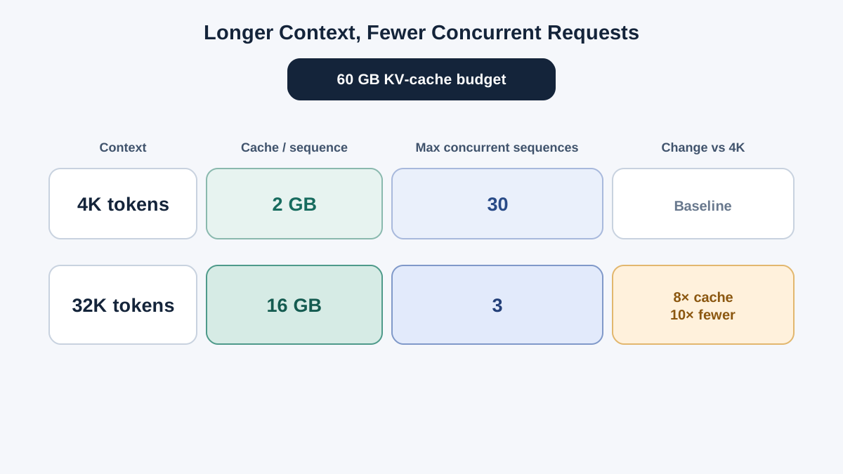
Now carry the earlier numbers through it. Suppose the GPU has of usable memory, the weights and runtime overhead consume , and each sequence runs at tokens. From the worked example, one sequence costs about . The remaining budget is , so:
Thirty requests at 4K tokens each. Push the same budget to tokens, where each sequence costs about , and the ceiling collapses to three concurrent sequences. Same hardware, same model, same weights — the only variable that moved was context length, and it cut concurrency by a factor of ten.
Run it in reverse and you get the other product decision: fix a target concurrency, solve for the maximum that still fits, and that number becomes your effective context limit regardless of what the model card advertises.
This is where batching meets memory. Larger batches raise throughput, but each additional sequence consumes cache, so the batch size is bounded by memory rather than by compute. The failure mode is specific and unpleasant: the scheduler admits one more request, memory runs out mid-generation, and the request either fails outright or forces eviction of another sequence's cache — which means recomputation, which means latency for a user who did nothing wrong.
Where the Simplified Model Breaks
The closed-form estimate is a planning tool, not a measurement. Know where it stops being accurate.
- Prefix sharing. If many requests carry the same prompt prefix, a serving stack with paged memory layouts can store that prefix once instead of once per request. The naive multiplier then overestimates cost for shared-context workloads.
- Eviction and compression. Dropping or compressing cached entries changes the effective or the effective bytes per element. These techniques trade memory against output quality in ways the formula cannot predict.
- Offloading. Moving cache to host memory or disk relieves capacity pressure but adds transfer latency. It changes the shape of the constraint rather than removing it.
- Cache quantization. Fewer bytes per element lowers the total, but approximation error compounds across decode steps.
- Sliding-window and sparse attention. These cap the effective cached length, which is why the linear-in- assumption is architecture-dependent, not universal.
Tip: Use the closed-form estimate for capacity planning and admission control. Measure real usage before you trust it as a hard limit.
What to Do With the Number
Read the model configuration to get , , and rather than guessing. Then decide which constraint you are actually solving for. Fixing context length and deriving concurrency produces a different product decision than fixing concurrency and deriving context length — pick the one that matches how your users behave.
Treat the estimate as an admission-control input. Reject or queue requests that would exceed the budget instead of discovering the limit through out-of-memory failures at 3 a.m.
And recognize when the exercise is overkill. Short-context, low-concurrency workloads rarely need this arithmetic. Optimizing cache memory before you have a concurrency problem is wasted effort.
The cache is per-request state that scales with tokens times concurrency, and that is why long context and high concurrency cannot both be free. Estimate bytes per token from the architecture, multiply by the workload, and treat the result as a budget you enforce — not a curiosity you compute after the outage. Your next concrete step: pull the config.json for the model you actually serve, plug its real layer count and head dimensions into the formula, and compare the result against the memory your serving stack reports. The gap between the two is where your operational margin lives.
Knowledge check
Final check
Finish the article by checking the ideas you just learned.
References
Want a more structured LLMOps path?
Use the LLMOps Practical Starter Bundle to connect RAG, evaluation, observability, and production patterns.
Large Language Models Starter Pack
A 12-chapter guide connecting LLM fundamentals with prompting, RAG, agents, tool calling, evaluation, security, and application engineering.
- 227-page Illustrated PDF edition
- 12 guided LLM engineering chapters
- Visual concept diagrams
- Self-assessment quizzes
- Bonus deep-dive sections
- Prompt design, structured output, context windows & RAG pipelines
- Agents, tool calling, prompt injection, evaluation & application lifecycles
Coming soon


