
Model LLM Cost, Latency, and Quality with Weighted Utility
Three engineers, three candidates, three different winners. The meeting ends the way it always does: whoever speaks last wins, and the decision gets…

Key topics
Three engineers, three candidates, three different winners. The meeting ends the way it always does: whoever speaks last wins, and the decision gets relitigated next sprint.
The tradeoff itself is not the problem. You already know that cheaper models tend to be faster and weaker, that bigger models tend to be slower and stronger, and that your token volume and request patterns decide how much any of that matters. That intuition is settled ground. What is missing is a way to combine three incomparable numbers into one comparable number — and to show your work while doing it.
A weighted utility score does not remove judgment from the decision. It forces judgment into the open, where it can be argued with, tested, and revised.
Why "Best Model" Is an Unfinished Sentence
When someone says "model A is best," they have silently finished a sentence that started with "given my priorities." The failure in the meeting is not that people disagree about facts. It is that each stakeholder is optimizing a different objective and calling it quality.
So start by naming the three raw metrics and their directions:
- Quality — higher is better. It must come from a defined evaluation, not vibes.
- Latency — lower is better.
- Cost — lower is better.
Direction matters because it determines the sign of every normalization you are about to write. Get a sign wrong and your "best" candidate becomes your worst.
The deliverable is a scalar per candidate, plus the ability to re-run it when assumptions move. That second part is the real product. A ranking you cannot re-derive is an opinion wearing a table.
Notation, Assumptions, and What the Score Can't Do
Before any arithmetic, define the pieces.
A candidate is one configuration — a model plus its settings — carrying a triple measured on a consistent basis. If one candidate's quality comes from a benchmark and another's comes from a colleague's impression, you are not comparing candidates. You are comparing measurement methods.
The bounds are , , , , , . These are chosen, not discovered. But there are two distinct ways to choose them, and mixing them up will quietly corrupt your comparison.
Candidate-derived bounds use the worst and best values in your current candidate set. If your three candidates have quality 8, 7, and 6, then and . This is the easiest policy, and it makes the best candidate score exactly 1.0 on that metric. The catch: add a fourth candidate at quality 10, and every existing quality utility shrinks. The frame moved, so the scores moved.
Fixed decision-range bounds come from outside the candidate set — a quality floor your product requires, a latency ceiling your users tolerate, a cost ceiling your budget allows. If you decide that quality 10 is the best value worth caring about and quality 6 is the worst acceptable, those bounds stay put even when the candidate set changes. A candidate at quality 8 then scores 0.5, not 1.0, because it occupies only part of the range you defined.
Both policies are legitimate. The mistake is switching between them mid-analysis, or reporting a score without saying which one produced it. For the rest of this article, the worked example uses candidate-derived bounds, and the bounds-sensitivity section switches to a fixed anchor on purpose — so you can see the difference.
The model rests on four assumptions:
- Metrics are commensurable after normalization.
- Preferences are stable across the decision.
- Weights are nonnegative and sum to one.
- The objectives are substitutable rather than hard constraints.
That fourth assumption is the one that bites. Linear additive utility assumes you will trade a little quality for a little latency at a constant rate. Often you won't — and we will break the model on purpose later to show where.
Note: Under candidate-derived bounds, the score is relative to the candidate set, not absolute. Add a new candidate and every existing score can shift. Under fixed bounds, scores stay anchored but may never reach 1.0.
Knowledge check
Check your understanding
Answer this question before you continue.
Deriving the Normalized Utilities
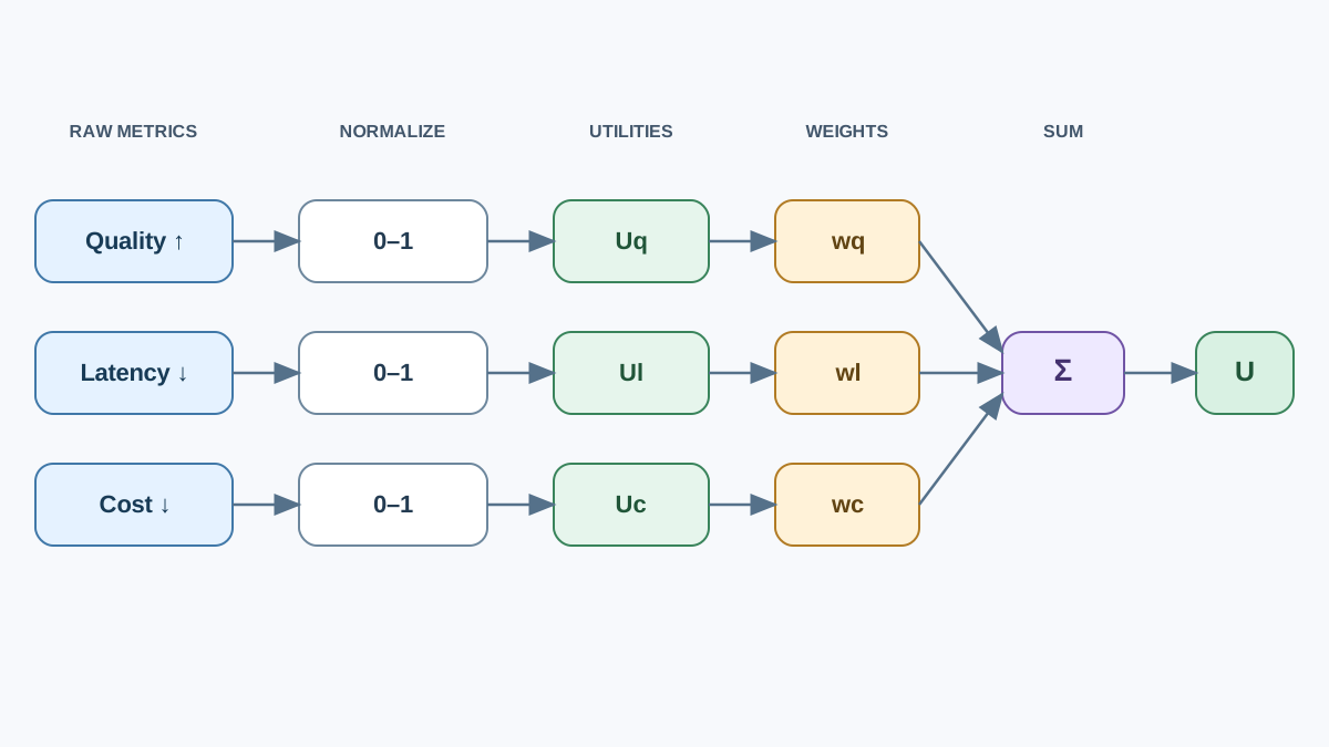
Raw units are incomparable. Milliseconds, dollars, and a 1–5 quality rating cannot be added. Normalization maps each metric onto a common scale where 0 is the worst value in the comparison range and 1 is the best.
Quality rises with the raw value, so the numerator measures distance above the floor:
The denominator is the width of the comparison range. A candidate at the top of the range gets 1; at the bottom, 0.
Latency falls as the raw value rises, so the numerator is inverted. Fast must map to 1, not 0:
Cost uses the same inversion for the same reason:
Every utility lands in . Now combine them:
The sum-to-one constraint is what makes the weights readable. means latency carries half of the total preference. Without the constraint, weights are arbitrary scale factors and you cannot compare two weight vectors at all.
Knowledge check
Check your understanding
Answer this question before you continue.
Worked Example: Three Candidates, One Ranking
Three hypothetical candidates, small numbers you can check by hand:
| Candidate | Quality | Latency (ms) | Cost (per 1K requests) |
|---|---|---|---|
| A | 8.0 | 900 | $4.00 |
| B | 7.0 | 300 | $2.00 |
| C | 6.0 | 150 | $0.50 |
Candidate-derived bounds: , , .
Normalize each metric:
| Candidate | |||
|---|---|---|---|
| A | |||
| B | |||
| C |
Now pick a starting weight vector for a latency-sensitive product: , , .
Candidate B, in full:
The other two:
Ranking: C (0.700) > B (0.664) > A (0.300). Candidate C wins, but only barely over B — and it wins on latency and cost, not quality. Candidate A, the quality leader, finishes last because it is the worst on both other metrics and the weights don't reward quality enough to compensate.
Knowledge check
Check your understanding
Answer this question before you continue.
Change One Weight, Watch the Ranking Move
Hold the raw values and bounds fixed. Change only the weights to reflect a cost-sensitive stakeholder: , , .
Ranking: C (0.700) > B (0.595) > A (0.300). The order holds, but the gap between C and B widens from 0.036 to 0.105. C is now more clearly the choice.
Push further. What if quality matters most — , , ?
Ranking: A (0.600) > B (0.574) > C (0.400). The winner flips. Candidate A, dead last under the latency-sensitive weights, takes first place once quality dominates.
The mechanism is simple: the ranking is a function of the weights. A ranking without stated weights is an incomplete claim. Report the weight vector alongside the winner, and test at least two plausible weight vectors before committing.
Knowledge check
Check your understanding
Answer this question before you continue.
Change the Bounds, Watch the Ranking Move Again
Bounds get less attention than weights and do just as much work. This time, switch to a fixed decision-range bound: suppose your product team has decided that quality 10 is the best value worth caring about, not quality 8. The candidates are unchanged. Only the anchor moved.
Keep the latency-sensitive weights (, , ) and set , .
New quality utilities: , , .
The order holds, but every quality utility compressed. A wider range stretches the denominator and squeezes candidates toward the middle. A narrower range does the opposite.
Now compare the two bound policies directly. Under candidate-derived bounds, A scored 1.00 on quality because it was the best in the set. Under fixed bounds anchored at 10, A scores 0.50 because it only reaches half the range you care about. Same candidate, same measurement, different frame — and a different score.
This is the quiet hazard. Under candidate-derived bounds, adding a very strong or very weak candidate to the comparison set silently changes every other candidate's score. No measurement changed. Only the frame did. Under fixed bounds, the scores stay stable, but you have to defend the anchor itself: why is 10 the ceiling and not 8 or 12?
Common mistake: Mixing the two policies. If you derive bounds from the candidate set in one analysis and from external targets in the next, your scores are not comparable. Pick one policy, name it in your report, and stay consistent.
What the Single Scalar Hides
The score is a preference aggregator, not a decision-maker. Four things it will happily hide from you:
Hard constraints are not preferences. A latency ceiling or a compliance requirement is a gate, not a weight. Filter candidates first, then score the survivors. A candidate that violates a constraint should never enter the arithmetic.
Distinct objectives can be non-substitutable. If two metrics must both clear a bar, an additive score will trade one away without complaint. The linear model cannot represent "both, or neither."
Quality is the softest input. If comes from a benchmark that does not match your workload, the score is precise about the wrong thing. Precision is not accuracy.
Averaging hides variance. Two candidates with the same can behave very differently under load. The score tells you the expected case, not the worst case.
A short checklist before you present a ranking:
- Filter on constraints.
- Score on preferences.
- Report weights, bounds, and the bound policy you used.
- Stress-test at least one weight and one bound.
The Decision Rule
Never present a ranking without its weights and its bounds. Those two choices are the argument. The arithmetic is just the receipt.
Take your own two or three real candidate configurations. Write down the bounds, the bound policy, and the weights before you score anything — that ordering is what keeps the numbers honest. Then run the sensitivity test on the weight you are least sure about, and watch whether the winner survives.
The point is not to end the disagreement. It is to make the disagreement visible, specific, and testable. "I think latency should carry more weight" is a claim you can now settle with a re-run instead of a re-meeting.
Knowledge check
Final check
Finish the article by checking the ideas you just learned.
Want a more structured LLMOps path?
Use the LLMOps Practical Starter Bundle to connect RAG, evaluation, observability, and production patterns.
Large Language Models Starter Pack
A 12-chapter guide connecting LLM fundamentals with prompting, RAG, agents, tool calling, evaluation, security, and application engineering.
- 227-page Illustrated PDF edition
- 12 guided LLM engineering chapters
- Visual concept diagrams
- Self-assessment quizzes
- Bonus deep-dive sections
- Prompt design, structured output, context windows & RAG pipelines
- Agents, tool calling, prompt injection, evaluation & application lifecycles
Coming soon


