
LLM Model Routing Break-Even Analysis: Work Through the Math
Routing is a bet on a classification. The break-even tells you the odds before you place it.

Key topics
Routing is a bet on a classification. The break-even tells you the odds before you place it.
You turn on routing. The bill drops. Three weeks later, support tickets describe answers that are confidently wrong. Nothing on the dashboard moved, because the dashboard measures spend, not the quiet degradation of the traffic you pushed downhill.
The weak mental model here is "routing saves money when most tasks are easy." That is true, and it is useless, because it never tells you how easy, or how much the classifier is allowed to cost, or what happens when it guesses wrong. The sharper model is this: routing pays only when the cost gap between routes clears the price of being wrong. That is a number you can compute before you write a single line of router code.
By the end of this article you will have one formula, one worked example with numbers you can swap for your own, and one failure mode that flips the sign of the whole result.
What You Are Actually Comparing
Before any arithmetic, name the two systems. A break-even needs a baseline to beat.
Baseline A sends every request to the strong model. Baseline B classifies each request, then routes it to a cheap or strong path.
The comparison is not "cheap model versus strong model." It is one policy versus another policy over the same traffic. That distinction matters, because the cheap model on its own is not a system — it is a component, and it has no opinion about which requests it should receive.
If you already know what a route and a fallback are, you have the prerequisite covered. The rest of this article assumes that vocabulary and does not re-teach it.
State your assumptions explicitly, because every one of them can break:
- A fixed traffic mix — the same distribution of easy and hard requests across the period you are modeling.
- A per-request cost for each route, including tokens in and out.
- A classifier that is neither free nor perfect. It costs something to run, and it will misroute some requests.
- A quality threshold you are unwilling to fall below.
There is a hidden third cost most builders forget: the classifier call itself, plus any escalation or retry that happens after a bad route. A request that goes cheap, fails, and then gets re-sent to the strong model pays both bills. If you leave that out of the model, your savings estimate is fiction.
Notation Before Arithmetic
Keep the symbol count small enough that the derivation stays readable. Six terms is enough.
Let p be the share of requests the classifier sends to the cheap route. This is a measured coverage number over all eligible requests, not the classifier's confidence score. A confidence threshold of 0.9 does not mean 90% of traffic goes cheap — it means you only send requests the classifier is 90% sure about, which could be 12% of traffic or 70% of it. Measure p; never infer it from a threshold.
Let C_cheap and C_strong be the expected per-request cost on each route, including input and output tokens.
Let C_classify be the per-request cost of making the routing decision. If your classifier is session-scoped — one decision for a whole conversation rather than one per turn — this amortizes across turns and shrinks fast.
Now separate quality from cost, because they behave differently. Let Q_cheap and Q_strong be pass rates against a stated threshold on a labeled set. Not "goodness." A pass rate. If you cannot write the threshold down, you cannot put quality into an equation, and you are back to vibes.
Common mistake: Treating p as the classifier's confidence. They are different numbers with different failure modes, and confusing them is how people build a router that routes 8% of traffic and wonder why the bill barely moved.
Knowledge check
Check your understanding
Answer this question before you continue.
Deriving the Cost Break-Even
Start with the baseline. Under the strong-only policy, expected cost per request is simply:
Cost_A = C_strong
Now build the routed policy term by term. Every request pays the classifier. Then a fraction p goes cheap, and the rest goes strong:
Cost_B = C_classify + p × C_cheap + (1 − p) × C_strong
Savings per request is the difference:
Savings = Cost_A − Cost_B
        = C_strong − C_classify − p × C_cheap − (1 − p) × C_strong
        = p × (C_strong − C_cheap) − C_classify
Set savings to zero and solve for the break-even proportion:
p* = C_classify / (C_strong − C_cheap)
In words: routing pays when the share of traffic you can safely send cheap exceeds the classifier cost divided by the per-request cost gap between routes.
Two consequences fall straight out of that division.
First, the degenerate case. If the strong route is not meaningfully more expensive than the cheap route, the denominator collapses and p* climbs past 1. No proportion of traffic makes routing pay. That is not an arithmetic error — it is a signal about your architecture. You picked two models that cost about the same, so there is nothing to arbitrage.
Second, the assumption that breaks first: a constant cost gap. Long-context requests and heavy-generation requests shift the gap in different directions, because input and output tokens are priced differently. If your traffic is bimodal — short chats and long document jobs — a single average gap will hide the fact that one segment is worth routing and the other is not.
Knowledge check
Check your understanding
Answer this question before you continue.
A Worked Example With Numbers You Can Swap
These figures are hypothetical and chosen so the division is checkable by hand. They are not vendor prices and not measured benchmarks.
Suppose a cheap route costs $0.002 per request, a strong route costs $0.020, and the classifier costs $0.0002.
p* = 0.0002 / (0.020 − 0.002)
   = 0.0002 / 0.018
   ≈ 0.011
About 1.1%. At these prices, routing pays if more than roughly one percent of your traffic is genuinely cheap-route traffic. That is a very low bar — which is the point. When the cost gap is ten-to-one, almost any real traffic mix clears it.
Now test two mixes. Take 100,000 requests.
| Traffic mix | p | Savings per request | Net savings |
|---|---|---|---|
| Mostly easy | 0.40 | 0.40 × 0.018 − 0.0002 = $0.0070 | $700 |
| Mostly hard | 0.005 | 0.005 × 0.018 − 0.0002 = −$0.00011 | −$11 |
The first mix clears the threshold comfortably. The second sits just below it, and the sign flips: routing now costs money, because you are paying the classifier on every request to send almost nothing downhill.
Notice the sensitivity. Halve the cost gap — say the strong route drops to $0.011 — and p* roughly doubles to about 2.2%. The cost gap moves p* far more than the classifier price does. In most realistic setups the classifier is a small fraction of the savings, so shaving classifier cost is rarely your leverage point. The traffic mix is.
Knowledge check
Check your understanding
Answer this question before you continue.
Adding Quality to the Equation
Cost alone will happily recommend a policy that answers half your users wrong. Add quality.
The expected quality of the routed policy is a weighted blend using the same p:
Q_routed = p × Q_cheap + (1 − p) × Q_strong
If the cheap route passes 80% of requests against your threshold and the strong route passes 95%, then at p = 0.40:
Q_routed = 0.40 × 0.80 + 0.60 × 0.95 = 0.89
You traded five points of pass rate for the savings. Whether that trade is acceptable is a product decision, not a math one — but now it is a visible decision instead of an accident.
The part most cost models omit: a failed answer is not free. A wrong answer routed cheap is a cheap call plus a support ticket, a retry, or a human review. Price that failure cost as a separate term and the effective cost of the cheap route rises:
C_cheap_effective = C_cheap + (1 − Q_cheap) × C_failure
That larger effective cost shrinks the gap, pushes p* upward, and can erase the savings entirely. If a failure costs $0.50 and the cheap route fails 20% of the time, the effective cheap cost is $0.002 + $0.10 = $0.102 — more expensive than the strong route it was supposed to replace.
My editorial judgment here is simple: I would rather run a slightly more expensive routing policy that holds quality than a cheaper one that quietly degrades answers. Silent quality regression shows up as tickets, not dashboards, and by the time the tickets arrive you have lost the trust you were trying to buy with the savings.
Knowledge check
Check your understanding
Answer this question before you continue.
When the Classifier Gets It Wrong
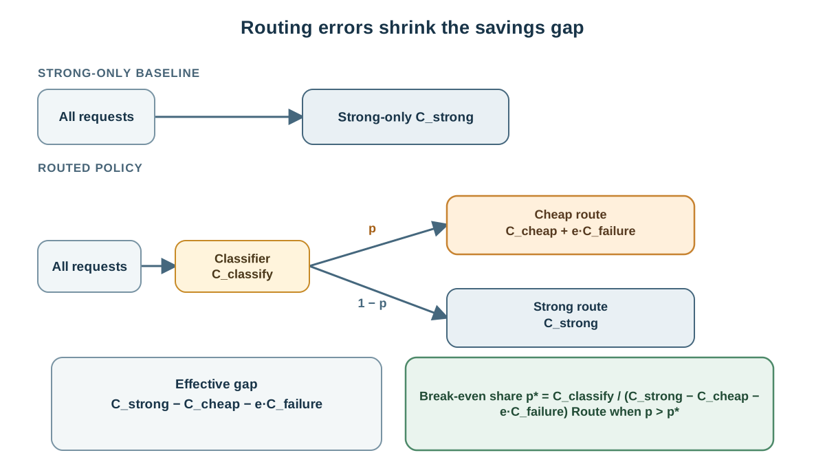
This is where the earlier result reverses. Classification errors, not model prices, decide whether routing wins.
Separate the two error types, because they cost different things:
- Under-routing — a hard request sent cheap. Costs quality, generates failure cost, and is the error that produces support tickets.
- Over-routing — an easy request sent strong. Costs money and quietly eats the savings, but nobody complains.
Here is the trap. It is tempting to say that a misrouted request "should not have gone cheap," so it no longer counts as cheap traffic. That is wrong, and it is the single most common way this analysis goes off the rails. A misrouted request still goes to the cheap route. The classifier's mistake does not move it back to the strong model. It still pays C_cheap. It still pays C_classify. The route share p is unchanged by the error rate.
What changes is the outcome of that request. Some fraction of cheap-routed requests will fail your quality threshold, and each failure carries a cost. So keep p as the actual route share, and add the failure penalty as its own term.
Let e be the under-routing rate: the fraction of cheap-routed requests that should have gone strong. Let C_failure be the expected cost of one such failure — the retry, the review, the ticket, the lost trust you can actually price. The expected cost of the routed policy becomes:
Cost_B = C_classify + p × (C_cheap + e × C_failure) + (1 − p) × C_strong
And the savings condition becomes:
Savings = p × (C_strong − C_cheap − e × C_failure) − C_classify
Solve for the break-even route share:
p* = C_classify / (C_strong − C_cheap − e × C_failure)
Read the denominator carefully. The error term e × C_failure does not shrink p. It shrinks the gap. Every misrouted request still costs you the cheap call; it just also costs you the failure. As e rises, the effective gap narrows, p* climbs, and at some error rate the denominator goes to zero — routing can never pay, no matter how much traffic you send downhill.
Now run the numbers. Keep the favorable mix, p = 0.40, C_cheap = $0.002, C_strong = $0.020, C_classify = $0.0002. Add a failure cost of $0.50 per under-routed request.
| Under-routing rate e | Effective gap | Savings per request | Net savings (100k) |
|---|---|---|---|
| 0% | $0.018 | $0.00700 | $700 |
| 15% | $0.018 − 0.15 × $0.50 = −$0.057 | −$0.0230 | −$2,300 |
| 60% | $0.018 − 0.60 × $0.50 = −$0.282 | −$0.1130 | −$11,300 |
The sign flips hard. At a 15% under-routing rate with a $0.50 failure cost, the policy that looked like a $700 win is a $2,300 loss. The raw traffic mix looked great. The error rate decided otherwise.
Notice what did not happen: p stayed at 0.40 the whole time. The requests still went cheap. They just failed, and failure has a price. That is the mechanism the naive model hides.
Warning: The traffic mix is the number that looks good. The error rate is the number that decides. Measure e on labeled data before you trust the mix.
What the Math Does Not Cover
Bound the model honestly, or you will over-trust a two-route equation.
The equation assumes a stable traffic mix. Real mixes drift by hour, feature, and customer segment. A policy that pays on average can lose money every Tuesday.
It ignores latency, which is a separate axis. A route can be cheaper and slower, and the break-even says nothing about that trade.
It ignores supervision and evaluation cost — building the labeled set, training or tuning the classifier, and maintaining it. That is an upfront expenditure that has to be recovered before any serving-time savings count. A routing policy that saves $700 a month but cost three engineer-weeks to build has a payback period you should compute before you celebrate the monthly number.
It assumes one cheap route and one strong route. Cascades and multi-tier routing need a branch table, not a single p.
Your Next Move: Measure p and e Before You Build
Before writing any router, label a few hundred representative requests. Estimate two numbers directly: p, the share that a cheap route could genuinely handle, and e, the under-routing rate you would expect from your classifier. Then price C_failure honestly — what does one bad answer actually cost you in retries, reviews, or churn?
Plug all three into the break-even condition and check the sign before committing engineering time.
If the sign is negative, the honest conclusion is that routing is not your leverage point yet. The cost gap, the traffic mix, or the classifier accuracy has to change first — pick models with a wider price spread, or accept that your workload is genuinely hard.
If the sign is positive, the next step is a bounded experiment: run a fixed set of tasks through both routes, compare measured quality, latency, and cost against explicit thresholds, and decide from the results rather than from the model.
Routing is a bet on a classification. The break-even tells you the odds. Compute them first, and you will know whether you are placing a bet or buying a lottery ticket.
Knowledge check
Final check
Finish the article by checking the ideas you just learned.
References
Want a more structured LLMOps path?
Use the LLMOps Practical Starter Bundle to connect RAG, evaluation, observability, and production patterns.
Large Language Models Starter Pack
A 12-chapter guide connecting LLM fundamentals with prompting, RAG, agents, tool calling, evaluation, security, and application engineering.
- 227-page Illustrated PDF edition
- 12 guided LLM engineering chapters
- Visual concept diagrams
- Self-assessment quizzes
- Bonus deep-dive sections
- Prompt design, structured output, context windows & RAG pipelines
- Agents, tool calling, prompt injection, evaluation & application lifecycles
Coming soon


