
Practice Finding a Pareto Frontier for LLM Tradeoffs
Six configurations sit on the whiteboard. Someone reaches for a single score to rank them, and the interesting part of the decision disappears.

Key topics
Six configurations sit on the whiteboard. Someone reaches for a single score to rank them, and the interesting part of the decision disappears.
Here is the move I want you to practice instead: before you weight anything, find the frontier. The frontier is the set of options that are still genuinely different bets. Everything else is a configuration you can delete without losing a single tradeoff.
This is a hands-on exercise. You will work one small synthetic table, mark the dominated rows, read the surviving frontier, then change one constraint and watch the answer move. The numbers are invented to produce a useful mix of dominated and non-dominated points. They do not describe any real provider, and they are not a recommendation.
If you have not yet read the prerequisite piece on cost, latency, and quality tradeoffs, the short version is enough: those three objectives pull against each other, and you cannot maximize all of them at once. That article explains why the tension exists. This one is about executing the comparison.
The Fixture: Seven Configurations, Three Objectives
| Config | Quality score (higher is better) | p95 latency, ms (lower is better) | Cost per 1k requests, $ (lower is better) |
|---|---|---|---|
| A | 71 | 900 | 4.20 |
| B | 78 | 1400 | 6.50 |
| C | 74 | 1100 | 5.10 |
| D | 82 | 2100 | 9.80 |
| E | 69 | 800 | 3.40 |
| F | 76 | 1300 | 7.90 |
| G | 73 | 1200 | 6.80 |
Three columns, three directions. Quality goes up. Latency goes down. Cost goes down.
Common mistake: Flipping a metric direction changes every dominance verdict in the table. If you treat "lower latency" as "higher is better" without inverting it, you will confidently eliminate the wrong rows. Write the direction next to each column before you compare anything.
The numbers are synthetic and deliberately small. Seven rows is enough to practice the procedure and small enough that you can check every pair by hand. This table stays fixed for the rest of the exercise — every result below is computed from exactly these values.
What Dominance Actually Means
A configuration is dominated when another configuration is at least as good on every objective and strictly better on at least one.
That is the whole rule. Two conditions, both required.
Walk one pair by hand. Compare A and C:
- Quality: C (74) beats A (71).
- Latency: A (900 ms) beats C (1100 ms).
- Cost: A ($4.20) beats C ($5.10).
C wins one column, A wins two. Neither dominates the other. Both stay live for now.
Now compare A and E:
- Quality: A (71) beats E (69).
- Latency: E (800 ms) beats A (900 ms).
- Cost: E ($3.40) beats A ($4.20).
Again, a split. A wins quality, E wins latency and cost. No domination.
Here is the trap. A configuration that wins on quality but loses on both latency and cost is not dominated. It is a different bet. It stays on the table until a constraint or a weight removes it. Beginners often delete the expensive high-quality option because it "feels worse." It is not worse. It is the only row that buys you that quality level.
Knowledge check
Check your understanding
Answer this question before you continue.
Step 1: Mark the Dominated Rows
Run this routine for each configuration:
- Pick a row.
- Scan every other row.
- Ask: does any single row beat this one on all three metrics, with at least one strict win?
- If yes, mark the row dominated and record which row beat it and on what.
Work it through. Start with B (78, 1400, $6.50). Scan the table. D has higher quality (82) but worse latency and cost. A is cheaper and faster but lower quality. C is cheaper and faster but lower quality. No single row beats B on all three. B survives.
Now C (74, 1100, $5.10). Compare against B: B has higher quality (78), but worse latency (1400 vs 1100) and worse cost ($6.50 vs $5.10). Split. Compare against A: A is faster and cheaper but lower quality. Split. C survives.
Now F (76, 1300, $7.90). Compare against B:
- Quality: B (78) beats F (76).
- Latency: F (1300) beats B (1400).
- Cost: B ($6.50) beats F ($7.90).
Split again. F survives.
Now D (82, 2100, $9.80). Highest quality in the table. Nothing beats it on quality, so nothing can dominate it. D survives by construction.
Now G (73, 1200, $6.80). Compare against C (74, 1100, $5.10):
- Quality: C (74) beats G (73).
- Latency: C (1100) beats G (1200).
- Cost: C ($5.10) beats G ($6.80).
C beats G on all three, with strict wins everywhere. C dominates G. G is eliminated, and you can delete it from the whiteboard without losing a tradeoff.
That leaves A and E. Compare A (71, 900, $4.20) against E (69, 800, $3.40):
- Quality: A (71) beats E (69).
- Latency: E (800) beats A (900).
- Cost: E ($3.40) beats A ($4.20).
Split. A survives. E survives by the same logic in reverse.
Note: A near-miss deserves a caveat. If two rows differ by a hair on one metric — say 1100 ms versus 1120 ms — do not declare a confident verdict. Small differences can be measurement noise. Note the pair and move on.
Knowledge check
Check your understanding
Answer this question before you continue.
Step 2: Read the Frontier
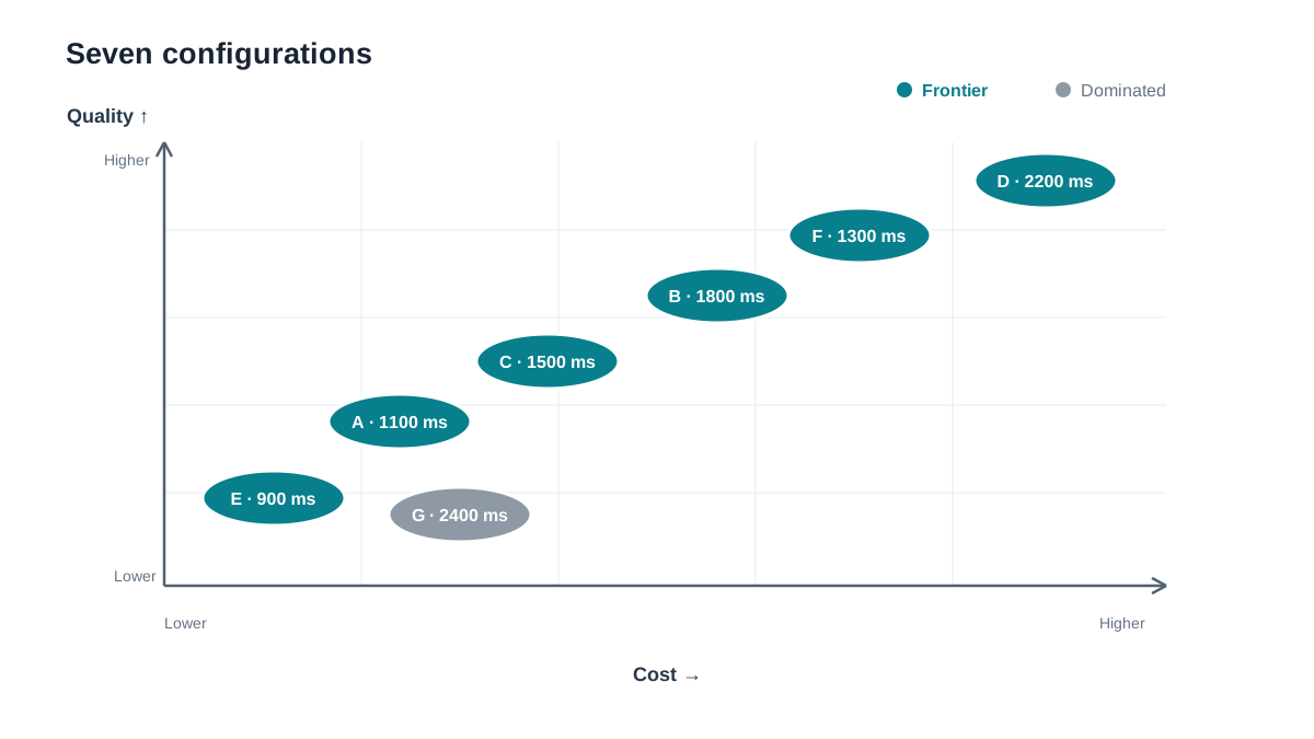
The surviving set is A, B, C, D, E, and F. Six non-dominated configurations. Read them left to right by quality:
| Config | Quality | p95 latency, ms | Cost per 1k, $ |
|---|---|---|---|
| E | 69 | 800 | 3.40 |
| A | 71 | 900 | 4.20 |
| C | 74 | 1100 | 5.10 |
| F | 76 | 1300 | 7.90 |
| B | 78 | 1400 | 6.50 |
| D | 82 | 2100 | 9.80 |
The broad shape is what you would expect: as quality rises, latency and cost tend to rise with it. But the marginal trade is not uniform, and one step breaks the pattern. Walk the steps:
- E to A: +2 quality for +100 ms and +$0.80.
- A to C: +3 quality for +200 ms and +$0.90.
- C to F: +2 quality for +200 ms and +$2.80.
- F to B: +2 quality for +100 ms and −$1.40 (B is cheaper than F).
- B to D: +4 quality for +700 ms and +$3.30.
That F-to-B step is the interesting one. B is both higher quality and cheaper than F, but slower. F is only on the frontier because of its latency. If your application does not care about the 100 ms difference, F is a poor deal — but it is not dominated, because latency is a real objective and F genuinely wins that column.
A two-axis view helps here: plot quality on the vertical axis and cost on the horizontal, then annotate each point with its latency. The frontier traces a curve from bottom-left (E) to top-right (D), with F sitting slightly off the cost curve because its value is speed, not price.
The key point: the frontier does not rank its own members. It tells you which choices are still live. It does not tell you which one to pick.
Knowledge check
Check your understanding
Answer this question before you continue.
Step 3: Change One Constraint and Recompute
Feasibility is a separate question from dominance. Dominance is a property of the metrics. Feasibility is a property of your requirements.
Suppose your product has a hard p95 latency ceiling of 1200 ms. Apply it to the frontier:
| Config | Latency | Feasible under 1200 ms? |
|---|---|---|
| E | 800 | Yes |
| A | 900 | Yes |
| C | 1100 | Yes |
| F | 1300 | No |
| B | 1400 | No |
| D | 2100 | No |
The frontier shrinks from six members to three. F, B, and D are now infeasible — not dominated, just unavailable. Their metric values did not change. Your requirement did.
Now check whether any previously dominated row becomes relevant. G was dominated by C, and C is still feasible, so G stays eliminated. But imagine the constraint had been a cost cap of $5.00 instead. Then C ($5.10) would be infeasible, and G ($6.80) would still be infeasible — but a different row might resurface. The lesson holds: when a constraint removes a dominator, re-run the dominance check on what remains.
Warning: If the constraint eliminates the entire frontier, your requirement set is unsatisfiable. That is a real signal, not a bug. Something has to give: relax the latency ceiling, accept higher cost, or lower the quality bar. Do not pretend a dominated row is now optimal just because it is the only one left.
Knowledge check
Check your understanding
Answer this question before you continue.
Why This Frontier Is Not a Recommendation
The frontier you just computed is conditional on four things: the metric directions, the metrics you chose, how you defined them, and the constraint you applied. Change any one and the answer moves.
Latency is the clearest example. A p95 time-to-first-token measurement and a p95 total-latency measurement produce different frontiers from the same system. If your users judge responsiveness by when the first token appears, TTFT is the metric that matters. If they wait for the full answer, total latency is. Pick the wrong one and you optimize the wrong curve.
The fixture is also synthetic and small. Real comparisons need consistent measurement conditions — same hardware, same load, same prompt distribution — and an awareness that small metric gaps can be noise rather than signal.
The durable rule: the frontier narrows the decision; it does not make it. Weighting and constraints still belong to the person with the requirement. That is the next step, and it is a separate exercise.
Your Turn: Extend the Fixture
Add a seventh configuration, H, with quality 80, latency 3000 ms, and cost $4.00. Predict where it lands before you check.
Work the comparisons explicitly. Against D (82, 2100, $9.80): D wins quality, H wins latency and cost — split, so D does not dominate H. Against B (78, 1400, $6.50): B wins latency and quality, H wins cost — split, so B does not dominate H. Against E (69, 800, $3.40): E wins latency and cost, H wins quality — split, so E does not dominate H. No single row beats H on all three metrics, so H is non-dominated. It is a genuine different bet: cheap and high-quality, but the slowest option in the table.
Then add a fourth objective, such as output token variance or memory footprint, and re-run the dominance check. Watch how quickly the frontier changes shape when you add a dimension. More objectives usually mean more surviving rows, because it becomes harder for any single configuration to beat another on every column.
Finally, flip one metric direction by mistake — treat cost as "higher is better" — and re-run Step 1. Feel how fast a careless sign error rewrites the answer. That is the failure mode this exercise exists to prevent.
Once the frontier is clear, the weighted-utility approach is the natural next move: assign weights to quality, latency, and cost, normalize each metric, and compute a single score. But do that after you know which options are live. Find the frontier first. Apply constraints second. Weight last.
Knowledge check
Final check
Finish the article by checking the ideas you just learned.
References
Want a more structured LLMOps path?
Use the LLMOps Practical Starter Bundle to connect RAG, evaluation, observability, and production patterns.
Large Language Models Starter Pack
A 12-chapter guide connecting LLM fundamentals with prompting, RAG, agents, tool calling, evaluation, security, and application engineering.
- 227-page Illustrated PDF edition
- 12 guided LLM engineering chapters
- Visual concept diagrams
- Self-assessment quizzes
- Bonus deep-dive sections
- Prompt design, structured output, context windows & RAG pipelines
- Agents, tool calling, prompt injection, evaluation & application lifecycles
Coming soon


