
Estimate the Memory a Local LLM Needs
Two people run the same 7B model. One says it needs 4 GB. The other says it needs 9 GB. Neither is lying.

Key topics
Two people run the same 7B model. One says it needs 4 GB. The other says it needs 9 GB. Neither is lying.
That gap is the whole problem. "Model size" feels like one number, so we treat memory as one number too. It isn't. Memory is a sum of parts, and once you can name the parts, you can estimate them in your head before you download a single gigabyte.
Here's the deal: you'll get a formula for the predictable part, a separate allowance for the messy part, and a clear statement of what the estimate cannot tell you.
Why One Memory Number Is Always Wrong
Ask "how much memory does this model need?" and you've asked a question with no single answer. The same model produces different figures because three things change underneath the label:
- Precision — how many bits each stored parameter occupies.
- Context length — how much text the model must hold in working memory at once.
- Runtime — the software loading the model, plus whatever else your machine is doing.
Change any one and the number moves. That's why the 4 GB person and the 9 GB person can both be right about the same weights.
So split the question in two:
- Weights — the learned values the model must load. Fixed for a given model and precision, and predictable.
- Runtime overhead — the working room the system needs on top. Variable, and workload-dependent.
If you've read our piece on what parameters actually are, you already know parameter count is an incomplete signal for capability. Here it becomes a genuinely useful sizing input — once you pair it with precision. Parameters tell you how much there is to store. Precision tells you how tightly it's packed.
One scope note before the math: this is a capacity screen for one user running one model. It is not a serving model for many concurrent requests. Keep that boundary in mind, because it's exactly where the simple version stops working.
The Two Numbers You Actually Need
Before any formula, let's name the inputs. There are only two.
P — parameter count. The number of learned values in the model. A "7B" model has P ≈ 7,000,000,000. That's it. No mystery.
b — effective weight bits. How many bits each stored parameter occupies at load time. Common values:
- 32 for full precision
- 16 for half precision
- 8 or 4 for common quantized formats
The word effective is doing real work there. Quantization doesn't always deliver exactly b bits per parameter once you count metadata and any layers the runtime keeps at higher precision. Treat b as the label on the box, not a guarantee about every byte inside it.
Where do you find these? The model card or config file gives you P and the storage type. The quantization label in the filename — something like Q4 — gives you b.
One assumption to state up front: every parameter is stored at the same precision. That's a simplification. We'll come back to where it breaks.
Knowledge check
Check your understanding
Answer this question before you continue.
Deriving the Weight Estimate
Let's build the formula one step at a time, because each step is just unit conversion.
Step 1: one parameter. A parameter stored at b bits occupies b/8 bytes. The division by 8 is nothing more than bits-to-bytes. One byte holds eight bits.
Step 2: all parameters. Multiply by P:
Step 3: convert to gigabytes. Here's a trap. Decimal gigabytes (10⁹ bytes) and binary gibibytes (2³⁰ bytes) differ by about 7%. Same number, different label, different answer. Pick one and stay consistent. I'll use decimal throughout.
Two anchors worth memorizing:
- Roughly 2 GB per billion parameters at 16-bit.
- Roughly 0.5 GB per billion at 4-bit.
Those two numbers will carry you through most quick comparisons.
Knowledge check
Check your understanding
Answer this question before you continue.
Worked Example: A 1B Model at 4 Bits
Let's run it end to end.
P = 1,000,000,000 and b = 4:
Half a gigabyte of idealized weights. Now the important part — what that 0.5 GB excludes:
- Quantization metadata such as per-group scales and zero-points.
- Embedding and output layers, which are often kept at higher precision.
- Any layers the runtime refuses to quantize.
This is why a real 4-bit download usually lands a bit above the idealized figure. The gap is metadata, not a mistake in your arithmetic. If your math says 0.5 and the file says 0.6, your math is fine.
The practical read: a 1B model at 4 bits is small enough that overhead, not weights, decides whether it fits comfortably. That flips your attention to the right place.
Knowledge check
Check your understanding
Answer this question before you continue.
Changing Precision Changes Everything
Same model, different b. The estimate scales linearly, so you can predict the result before computing it.
| Precision | Bytes per parameter | 1B model | 7B model |
|---|---|---|---|
| 32-bit | 4 | ~4 GB | ~28 GB |
| 16-bit | 2 | ~2 GB | ~14 GB |
| 8-bit | 1 | ~1 GB | ~7 GB |
| 4-bit | 0.5 | ~0.5 GB | ~3.5 GB |
Read the table as idealized weights only. Every cell needs overhead added before it means anything about fit.
Lower precision is not free. Aggressive quantization can change outputs, and it can even slow inference, because the runtime has to quantize and dequantize during decoding. Smaller is not automatically faster.
My decision rule: pick the highest precision that fits your memory budget with room left for overhead — not the smallest number that technically loads.
Adding Runtime Overhead Without Fooling Yourself
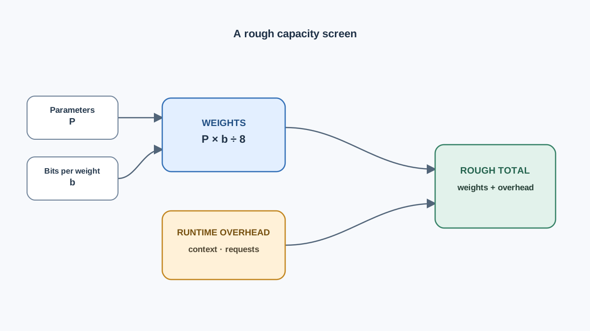
Now the second bucket. This is where most beginner sizing errors live, because the weight estimate feels like an answer and it isn't.
The largest runtime cost is usually the KV cache — the stored attention keys and values that let the model reuse previous tokens instead of recomputing them. It grows with context length and with how many requests are in flight at once.
Other overhead: temporary activations, framework and driver allocations, and a fragmentation buffer the allocator needs.
A common shortcut is a percentage multiplier on the weight estimate — often somewhere in the 10–30% range. Useful as a rough screen. Misleading as a precise model. The KV cache depends on sequence length, batch size, layer count, and hidden size, so long-context workloads can need far more headroom than a flat percentage suggests.
Let's apply that shortcut to the worked example so the two buckets actually combine. Start with the 0.5 GB of idealized weights for the 1B model at 4 bits. Choose a 20% overhead allowance — a stated assumption, not a universal requirement:
So the capacity screen says: plan for roughly 0.6 GB before you count the operating system, the runtime process, and anything else running on the machine. That is the number to hold against your available memory — not the 0.5 GB weight figure alone.
And keep the caveat attached. If you push context length up or run a second request, the real overhead can blow past that 20% allowance. The multiplier is a starting guess, not a ceiling.
Common mistake: Treating the weight estimate as the total requirement. Weights are the fixed block. Overhead is the block that grows while you're not looking.
Knowledge check
Check your understanding
Answer this question before you continue.
What the Estimate Cannot Tell You
Set the boundaries honestly, or you'll trust the number for jobs it can't do.
Fitting is not running well. Once weights are loaded, memory bandwidth often gates tokens per second more than raw capacity does. A model that fits can still crawl.
CPU offloading can fake a fit. Spilling layers to system RAM makes a model "fit" at a real cost in throughput. It loads. It may not be usable.
Hardware and software support vary. Not every GPU accelerates every precision format natively, so a format that fits may not be the fast path.
Treat the estimate as a capacity screen. It rules models out cheaply and tells you what to measure next. It does not tell you what performance you'll get.
Use it when shortlisting models before downloading tens of gigabytes. Don't use it for capacity planning across multiple users or long-context workloads — that's a different problem with different math.
Your Next Step: Screen, Then Measure
Run the formula on the two or three models you're actually considering, at the precision you'd realistically download. Write the weight estimate next to your available memory, add a stated overhead allowance on top, and leave explicit headroom instead of assuming zero.
The estimate tells you what to try. An actual run tells you what happens. Measure elapsed time and observed memory use on your own machine — and remember that measurements from one machine are observations, not benchmarks.
Weights are predictable. Overhead is not. Keep those two buckets separate and you'll stop being surprised by numbers that disagree. Then go run one and see what your hardware says.
Knowledge check
Final check
Finish the article by checking the ideas you just learned.
References
Want a more structured LLMOps path?
Use the LLMOps Practical Starter Bundle to connect RAG, evaluation, observability, and production patterns.
Large Language Models Starter Pack
A 12-chapter guide connecting LLM fundamentals with prompting, RAG, agents, tool calling, evaluation, security, and application engineering.
- 227-page Illustrated PDF edition
- 12 guided LLM engineering chapters
- Visual concept diagrams
- Self-assessment quizzes
- Bonus deep-dive sections
- Prompt design, structured output, context windows & RAG pipelines
- Agents, tool calling, prompt injection, evaluation & application lifecycles
Coming soon


