LLM Quantization Tradeoffs: What Lower Precision Changes

Two model files sit in your download folder. Both say 4-bit. One is smaller, one runs faster, and they give you different answers to the same prompt. If bit width were a single dial for size, speed, and quality, that should be impossible.

It isn't impossible. It's the normal case. "4-bit" is a label for a family of representation schemes, not a measurement. Once you see why, you can read a quantized model card without being fooled by the number in its name.

Why "4-bit" Is Not One Thing

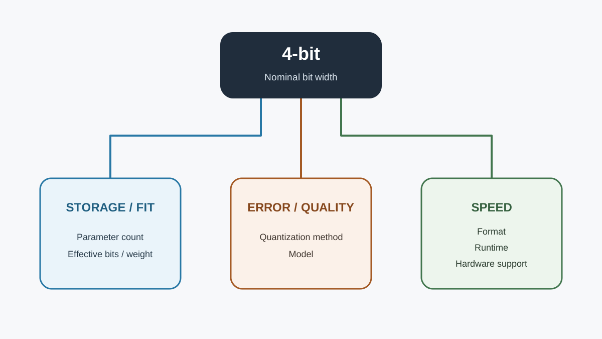
Here's the confusion in plain form: you pick a quantized model, you check the bit width, and you expect the rest to follow. Smaller number, smaller file, faster inference, slightly worse answers. A clean dial.

The dial model breaks the moment you compare two real files. They can share a nominal bit width and still differ in effective bits per weight, file size, and behavior. The reason is that quantization decisions live in three separate layers, and only one of them is about the number 4.

1. Idealized storage. How many bytes the weights would occupy if precision were uniform and nothing else existed.
2. Representation error. What rounding does to the values themselves, and how that error compounds through the network.
3. Implementation and hardware. Which format was used, whether your runtime has optimized kernels for it, and whether your GPU accelerates it at all.

Grant the dial model its narrow win: for a rough capacity screen before you download anything, P × b / 8 is genuinely useful. It tells you whether a model has a chance of fitting. That is the whole job it can do reliably.

The thesis of this article: nominal bit width is a label for a scheme, not a measurement of quality, speed, or compatibility. Storage, error, and implementation each follow different rules. Reason about them separately or you will misread every model card you touch.

Notation and Assumptions Before the Math

Before deriving anything, name the symbols.

• P — parameter count. The number of weights in the model.
• b — nominal bits per weight, as advertised. The "4" in 4-bit.
• M_weights — idealized weight storage in bytes.

The idealized relation is:

$M_{\text{weights}} \approx \frac{P \times b}{8} \text{ bytes}$

This deliberately excludes a lot. Quantization metadata — scales, zero-points, block overhead — is not counted. Neither is the KV cache, activations, or framework overhead. The estimate covers weights and only weights.

State the assumptions explicitly, because they are what make the formula clean and what make it incomplete:

• Uniform precision across layers. No mixed precision, no layers kept at higher bits.
• No sparsity. Every parameter is stored.
• Decimal gigabytes. We divide by $10^9$, not $2^{30}$. The convention matters when you compare against a file size on disk.

If you've already worked through the baseline memory estimate, this is the same relation — the focus here shifts from capacity to consequence. What does lower precision actually change once the file is on disk?

Deriving the Storage Relationship Step by Step

Start from the smallest unit. Each weight is stored using b bits. With P weights, the total bit count is:

$\text{total bits} = P \times b$

Convert bits to bytes by dividing by 8:

$M_{\text{weights}} = \frac{P \times b}{8} \text{ bytes}$

Scale to gigabytes by dividing by $10^9$:

$M_{\text{weights}} \approx \frac{P \times b}{8 \times 10^9} \text{ GB}$

Now watch it behave. Take a 7-billion-parameter model and step the precision down:

Nominal precision	b	Idealized weight storage
16-bit	16	≈ 14 GB
8-bit	8	≈ 7 GB
4-bit	4	≈ 3.5 GB

Each halving of b halves the storage. The relationship is linear in b, which is exactly why it works as a capacity screen and fails as a performance predictor. Linearity is a property of the storage model, not of the system.

Here's the first crack. Nominal b is not effective bits per weight. Real 4-bit schemes carry metadata — scales and zero-points stored alongside blocks of weights — so the true figure lands above 4. A file labeled 4-bit might store closer to 4.5 or 4.8 effective bits per weight. That gap is why the file you download is often larger than the formula predicts. The formula gives you a floor, not a promise.

Where the Idealized Estimate Breaks

Weight storage is not total memory. This is the mistake I see most often, and it costs people an afternoon of debugging an out-of-memory error they thought was impossible.

The KV cache, activations, and runtime buffers scale with context length and batch size, not with b. Quantizing weights does not shrink the KV cache. That is a separate decision requiring separate quantization. A model whose weights fit comfortably can still exhaust memory once you push a long context through it.

Picture a layered memory bar. The bottom layer is idealized weights — the part the formula describes. Stacked on top: the KV cache, activations, framework overhead. The formula only ever describes the bottom layer. Everything above it is invisible to the estimate.

And the estimate says nothing about latency or throughput. Speed depends on whether your hardware has kernels for the format. A format that saves memory may not be accelerated at all — which means it can be smaller and slower at the same time. That possibility is not a paradox. It's the implementation layer asserting itself.

Representation Error: What Rounding Actually Costs

Now the second layer. Uniform quantization maps a range of floating-point values onto a limited set of integer levels using a scale, an offset, and rounding. The reconstructed value is the integer level scaled back up. The difference between the original weight and its reconstruction is the quantization error.

That error compounds. A small per-weight error propagates through many layers, and the network's output reflects the accumulated drift, not any single rounding decision.

Error is not uniform across a model. Outlier weights and activations are harder to represent within a fixed range, which is why different quantization methods differ in what they protect — some preserve weights by activation magnitude, others smooth activation outliers before quantizing. The method matters as much as the bit width.

What does this look like in practice? Degradation shows up unevenly. Some tasks tolerate aggressive quantization well. Others — strict instruction adherence, precise formatting, long-context reasoning — are far less forgiving. Smaller models tend to suffer more at 4-bit than large ones. And hard tasks don't always lose the most; quantization tends to magnify a model's existing weaknesses rather than scale with task difficulty.

The consequence: a single bit-width number cannot predict quality. Two 4-bit models can land in different places because they used different methods, protected different values, and started from different base models.

Implementation and Hardware: The Layer Bit Width Hides

The third layer is where "4-bit" stops meaning anything on its own.

First distinction: weight-only versus weight-and-activation quantization. Weight-only schemes (often written W4A16) quantize the weights and leave activations at higher precision. Weight-and-activation schemes (W8A8) quantize both. They change different parts of the computation, so they carry different accuracy and speed profiles.

Second distinction: integer versus low-precision floating-point formats. The same nominal width can carry different dynamic range and precision depending on how the bits are split between exponent and mantissa. A 4-bit integer and a 4-bit float are not interchangeable.

Third, and decisive: hardware support is the gate. A format that saves memory may not be accelerated by your GPU. Compatibility is a property of the format-plus-runtime pair, not of the number 4 or 8. The same file can fly on one stack and crawl on another.

Common mistake: Assuming a lower bit width guarantees a speedup. If your runtime lacks optimized kernels for the format, you pay the quality cost without the speed benefit.

A Controlled Hypothetical Comparison

Here's a thought experiment that isolates the layers. It's a reasoning device, not a benchmark — real measurements are machine-specific.

Set up the comparison: hold the model, the runtime, the hardware, and the prompt fixed. Vary only the precision of the stored weights.

First pass — vary only representation error. Same format family, same kernels, different bit width. Go from 8-bit to 4-bit within one family. Any change in output quality is attributable to representation error, because nothing else moved. You've isolated layer two.

Second pass — hold bit width fixed, change the format or the runtime. Keep the nominal 4-bit label, but switch from one format family to another, or run it on a stack without optimized kernels. Any change in speed or output now comes from implementation and hardware, not from precision. You've isolated layer three.

The two passes produce different effects. That's the point. If nominal bit width were a single predictor, both passes would move the same needle. They don't. Precision changes representation error; format and runtime change speed and compatibility. Because these are separate causes, bit width alone cannot predict quality, speed, or compatibility.

Note: This experiment is for reasoning, not measurement. It tells you which variable to suspect. It does not tell you what your machine will do.

Reading a Quantized Model Card Without Being Fooled

Turn the three-layer model into a checklist. When you look at a quantized model, ask:

• What does the label specify? Nominal bit width, format family, weight-only versus weight-and-activation, and block or group size. "4-bit" alone answers none of these.
• What are the effective bits per weight? Once metadata is counted, the real figure sits above the nominal number. Compare it against the file size you actually see.
• Does your runtime and hardware accelerate that format? Check before assuming a speedup. This is the gate, not the bit width.
• Which tasks do you care about? Degradation is uneven. A general benchmark score may not cover your use case.

The decision rule: use the storage estimate to screen for fit, then test the specific format on your own hardware and task before committing. The formula gets you to a shortlist. Only a real run gets you to a decision.

When Lower Precision Is the Right Call — and When It Is Not

Reach for lower precision when memory or cost is the binding constraint and your task tolerates modest output variation. That's the common case, and it's why quantization is here to stay.

Be cautious when the task depends on strict instruction adherence, precise formatting, or long-context reasoning. These are the areas where degradation tends to be least forgiving.

Be cautious when your hardware lacks accelerated support for the format. You may pay the quality cost without the speed benefit — the worst of both.

Common mistake: Assuming a smaller quantized model always beats a larger full-precision one, or the reverse. The comparison depends on the task and the format. A 4-bit larger model can outperform a full-precision smaller one on most tasks while struggling with strict instruction following. Neither direction is a rule.

The Number Was Never the Answer

Return to the two files. Both said 4-bit. Now you can explain the difference: storage follows the idealized relation, quality follows representation error, and speed and compatibility follow implementation and hardware. Three layers, three different rules, one misleading label.

Your next move: pick one quantized model you're considering. Write down three things — its nominal bit width, its format family, and its effective bits per weight. Then check whether your runtime and hardware actually accelerate that format before you trust any speed or quality claim attached to it. The label tells you where to start looking. The layers tell you what you'll find.