
Practice Comparing Quantized LLM Outputs on a Fixed Task
You swap a model to a 4-bit build, run the same prompt, and get a slightly different answer. Now what? You cannot tell whether quantization degraded the…

Key topics
You swap a model to a 4-bit build, run the same prompt, and get a slightly different answer. Now what? You cannot tell whether quantization degraded the model or whether the model was always going to answer that way.
That uncertainty is the real problem, and it is not solved by running a bigger benchmark. It is solved by running a smaller, controlled one. One task, one prompt, two precision configurations, one observation table, and an honest reading of what the result does and does not prove.
What This Comparison Can and Cannot Prove
A benchmark is a result under agreed test conditions. This exercise is a single observation under your conditions. Those are different things, and confusing them is how beginners end up making confident claims from one afternoon of tinkering.
Your result will be specific to five things:
- The model — its size, architecture, and training.
- The quantizer and its settings — GPTQ, AWQ, bitsandbytes, GGUF k-quants, and others behave differently, and so do their configuration choices.
- The hardware — CPU versus GPU changes both memory patterns and latency.
- The workload — a format-heavy extraction task and a reasoning-heavy task stress the model differently.
- The sample — the specific prompts you chose.
Two configurations is enough to practice the method. It is not enough to rank quantization schemes. Quantization reduces weight precision — for example FP16 down to 8-bit or 4-bit — to cut memory and compute, and it can cost accuracy. How much depends on the setup, not on the bit count alone. Research on quantized models has generally found that larger models preserve output quality better than smaller ones under the same quantization, but that is a pattern across many evaluations, not a prediction about your run.
So say plainly what you will not claim at the end: no general quality verdict, no speed ranking, no recommendation for anyone else's hardware.
Prerequisites and the Fixture You Will Reuse
You already know how to run a small local model and record elapsed time and memory. You already know the weight-size estimate:
M_weights ≈ P × b / 8 bytes
where P is parameter count and b is effective weight bits. This article uses both as inputs, not as topics.
Now pin down the fixture so precision is the only variable.
Pick one small model and one task type. A short summarization task or a fixed-format extraction task with a checkable answer works well. Extraction is easier to score because you can verify field presence mechanically.
Choose two precision configurations of the same model family. A higher-precision build and a lower-precision build — for example an 8-bit and a 4-bit variant, or FP16 versus a 4-bit quantized build.
Record the exact model identifier, quantizer or quantization method, and any runtime flags. If you cannot name the quantizer, you cannot interpret the difference. "4-bit" is not a quantizer; it is a bit width.
Freeze everything else. Same runtime, same context length, same generation settings, same machine, same session where possible.
Note the hardware and whether inference runs on CPU or GPU. Memory and latency patterns differ sharply between them, and so does the meaning of your resource numbers.
Note: If you are using a runtime like Ollama, the model tag itself often encodes the quantization. A tag ending in
q4_K_Mand one ending inq8_0are two different quantizations of the same base model. Write both tags down verbatim.
Define the Task Criteria Before You Run Anything
This is the step beginners skip, and it is the step that makes the rest of the exercise work. Without criteria written in advance, every output difference looks like a quality difference. The more fluent-sounding answer wins, regardless of whether it is correct.
Write three to five checkable criteria for your task. For an extraction task, that might look like:
- The output contains all required fields.
- The output is valid JSON (or your target format).
- The key fact or value is correct.
- The output length is within bounds.
Separate criteria that are mechanically checkable — format, field presence, exact value — from criteria that require judgment, like tone or completeness. Decide in advance how you will score each one. Pass/fail is enough. A five-point scale invites false precision, and you will spend more time arguing with yourself about whether something is a 3 or a 4 than you will spend learning anything.
Write the prompt once and save it verbatim. Do not rewrite it between runs, even to "help" the weaker configuration. The moment you adjust the prompt after seeing a bad output, you are no longer comparing precision configurations. You are comparing two different experiments.
If the task has a reference answer, note it now, so you can compare outputs against something other than each other.
Knowledge check
Check your understanding
Answer this question before you continue.
Run Both Configurations and Capture the Same Fields
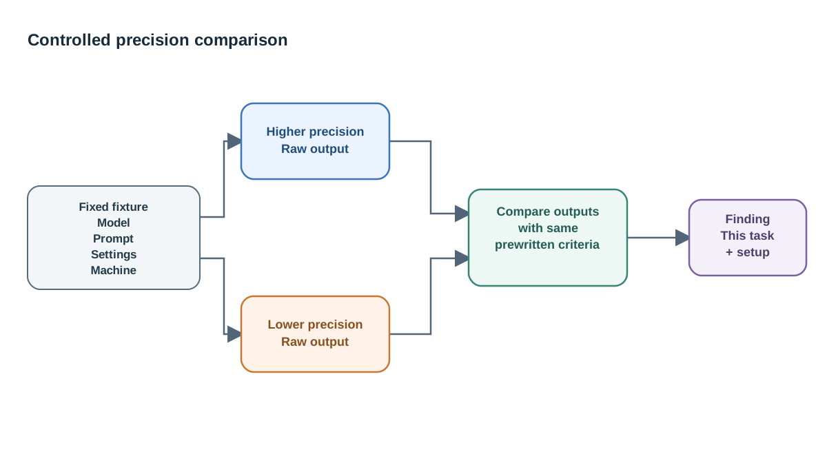
Run the higher-precision configuration first, then the lower-precision one, using the identical prompt and generation settings.
Capture the same fields for both runs:
| Field | Run A (higher precision) | Run B (lower precision) |
|---|---|---|
| Model identifier | ||
| Quantization / precision | ||
| Prompt (verbatim) | ||
| Raw output | ||
| Elapsed time | ||
| Memory observation | ||
| Repeat-stable? |
Record the output verbatim. Do not clean it up, trim it, or paraphrase it. The differences you are hunting live in the raw text — a dropped field, a stray token, a changed number. If you tidy the output before saving it, you erase the evidence.
Run each configuration more than once if your runtime allows it, and note whether the output is stable across repeats. Instability is itself a finding. A configuration that gives you a different answer every time is telling you something about the task, the sampling settings, or the model — and that is worth knowing before you attribute anything to precision.
Common mistake: A 4-bit build may report a different parameter count or tensor shape than the higher-precision build. This is not the model changing. Quantized weights are packed — in a 4-bit scheme, one byte can hold two parameters — so the reported shape reflects the storage format, not a different network. Do not let this send you down a debugging rabbit hole.
Keep one table with one row per run and one column per field. The comparison should be mechanical, not remembered.
Knowledge check
Check your understanding
Answer this question before you continue.
Read the Output Differences Against Your Criteria
Now turn two blocks of text into an interpretation. This is where most beginners stop at "they look similar" and miss the actual signal.
Score each run against the criteria you wrote earlier. If you can manage it, score before you look at which configuration produced which output — it removes the temptation to grade generously toward the one you expect to win.
Then classify each difference into one of four buckets:
- Formatting drift — same content, different structure.
- Wording variation — same meaning, different words.
- Missing or extra content — a field dropped, a sentence added.
- Factual or logical error — a wrong value, a broken inference.
The distinction that matters most is between meaning-preserving variation and meaning-changing error. Word choice and structure can shift while the answer stays correct. A dropped field or a wrong value is a different category entirely, and it is the one your criteria should catch.
Look specifically for the failure that hurts most: a confidently wrong answer that still passes your format checks. Valid JSON with the wrong number inside is worse than malformed JSON, because it looks trustworthy.
Note where the lower-precision run failed a criterion the higher-precision run passed. Also note where it passed one the higher-precision run failed. That happens, and recording it honestly is part of the discipline.
Compare resource observations alongside quality. Less memory and faster generation are the expected trade, but confirm it on your machine rather than assuming it. If the lower-precision run was not actually faster or smaller in your setup, that is a finding worth writing down.
Knowledge check
Check your understanding
Answer this question before you continue.
Common Mistakes That Invalidate the Comparison
These are the specific ways this experiment quietly stops being a comparison:
- Changing the prompt between runs, or "fixing" it after seeing the weaker output.
- Comparing different model sizes or different model families and attributing the difference to precision.
- Comparing across different runtimes, context lengths, or generation settings without recording the change.
- Judging quality by feel instead of against pre-written criteria.
- Treating one prompt as a representative sample of the model's behavior.
- Reporting a single latency or memory number as a benchmark when it is one observation on one machine under one workload.
Each of these mistakes has the same shape: you changed more than one thing and credited the difference to the thing you were curious about. Controlled comparison is mostly the discipline of not doing that.
Knowledge check
Check your understanding
Answer this question before you continue.
Extend the Experiment: One Meaningful Change
A single comparison gives you a data point. A follow-up tells you whether that data point means anything.
Pick one change:
Add a third configuration. A different bit width or a different quantizer. Does the pattern hold, or does it break? If 8-bit and 4-bit look similar but a different 4-bit method diverges, you have learned that the quantizer matters more than the bit count for this task.
Hold precision constant and change the task. Move from a format-heavy task to a reasoning-heavy one. If the gap between configurations widens, you have evidence that precision loss shows up more in some workloads than others.
Repeat the same task across several prompts of the same type. If the difference is consistent, it is a pattern. If it is a one-off, it is noise.
Before you run the follow-up, predict the outcome. Write it down. Then compare your prediction with the result. The gap between the two is the actual lesson — it tells you which part of your mental model of quantization needs updating.
Record what would have to change before you could make a stronger claim: more prompts, more configurations, a different machine, a second quantizer.
How to Report What You Found
Close the loop by stating a finding with its scope attached. This is the durable skill the exercise is really building.
Write the finding in one sentence that names the model, the two configurations, the task, and the hardware. Something like: "On this machine, running this model at 8-bit and 4-bit on a fixed extraction task, the 4-bit run dropped the second field in one of three attempts."
Then separate what you measured from what you inferred. "The 4-bit run dropped the second field" is measured. "4-bit is unreliable for extraction" is an inference that needs more evidence. Keep the two in different sentences, and you will avoid most of the overclaiming that surrounds quantization discussions.
Keep the table and the raw outputs. They are the reusable asset. The conclusion is the disposable part — you will replace it the next time you run the experiment on different hardware or a different model.
Before you trust any claim about a quantized model — including your own — ask three questions: What was held constant? What was measured? What was the sample? Those three questions will serve you every time you swap a model, a quantizer, or a runtime. Keep the observation table as a template, and run the next comparison the same way.
Knowledge check
Final check
Finish the article by checking the ideas you just learned.
References
Want a more structured LLMOps path?
Use the LLMOps Practical Starter Bundle to connect RAG, evaluation, observability, and production patterns.
Large Language Models Starter Pack
A 12-chapter guide connecting LLM fundamentals with prompting, RAG, agents, tool calling, evaluation, security, and application engineering.
- 227-page Illustrated PDF edition
- 12 guided LLM engineering chapters
- Visual concept diagrams
- Self-assessment quizzes
- Bonus deep-dive sections
- Prompt design, structured output, context windows & RAG pipelines
- Agents, tool calling, prompt injection, evaluation & application lifecycles
Coming soon


