
Hosted vs Local LLM Cost: Calculate the Break-Even Workload
Two people run the same break-even calculator, feed it the same hardware price, and get opposite answers. Both are right.

Key topics
Two people run the same break-even calculator, feed it the same hardware price, and get opposite answers. Both are right.
That is the first thing to understand about hosted vs local LLM cost break even: the crossover point is not a property of a GPU or an API. It is a derived quantity, and it moves the moment you change the horizon, the utilization, or the comparison target. Published thresholds range from roughly two million tokens per day to billions of tokens per month, and most of that spread comes from authors quietly comparing against different hosted tiers.
So we are not going to look up an answer. We are going to build a small model, solve it for the crossover volume, and then break our own assumptions to see whether the answer survives.
If you have not yet decided between hosted and local on criteria like privacy, control, and setup effort, that is a separate decision with its own logic. This article only prices the two paths.
Why Published Break-Even Numbers Disagree
Search for a break-even figure and you will find confident, incompatible numbers. The reason is not that someone did the arithmetic wrong. It is that three variables silently decide the answer, and most published thresholds state only one of them.
Monthly token volume. A workload doing 500,000 tokens a day and one doing 30 million tokens a day live in different economic worlds. Fixed local costs amortize across volume; hosted costs scale with it.
Which model tier the workload actually needs. This is the variable people skip. If your task runs fine on a small open-weight model, the honest comparison is a cheap hosted endpoint, not a frontier API. That single choice can move the crossover by more than an order of magnitude.
Workload type. Short API-style calls and long-context retrieval workloads consume very different amounts of compute per token. A retrieval-heavy workload with large context can cost several times more per million tokens to serve locally than a short chat call, which pushes the break-even volume higher.
A break-even point is a derived quantity. Change the horizon, the utilization, or the labor rate, and the crossover moves. The skill is not memorizing the number. The skill is constructing it.
Define the Model Before You Calculate
Before any arithmetic, write down what you are comparing. Here is the notation I use.
| Symbol | Meaning | Units |
|---|---|---|
V | Token volume through the system | tokens per month |
p | Hosted price for the comparison tier | dollars per million tokens |
H | One-time local cost: hardware, setup, hardening | dollars |
M | Recurring local cost: electricity, hosting, maintenance labor | dollars per month |
T | Planning horizon | months |
The two cost families behave completely differently, and that asymmetry is the whole article.
Hosted cost scales with volume and has no floor. At zero tokens, you pay zero. Double the volume, double the bill.
Local cost is mostly fixed and barely moves with volume. You buy the hardware once, you pay for power and maintenance every month, and the bill looks the same whether the box serves ten thousand tokens or ten million — until you hit its throughput ceiling.
State your horizon first. Twelve months is the common default, but it is not neutral: hardware amortizes over the horizon while API spend does not. A 36-month horizon lowers the effective monthly local burden and makes local look better. That is a real effect, not a trick, but you have to say which horizon you used.
Then name what you are deliberately holding constant:
- Model quality parity between the two paths
- No retry, failure, or re-processing overhead
- Stable hosted pricing across the horizon
- No capacity ceiling on the local box
That last one is a lie you are telling yourself temporarily. We will come back to it.
Warning: The biggest hidden assumption is that your workload can run on the local model at all. If it genuinely needs a frontier model, the comparison target changes, and the arithmetic changes with it. Test that assumption before you price anything.
Knowledge check
Check your understanding
Answer this question before you continue.
The Break-Even Equation, Step by Step
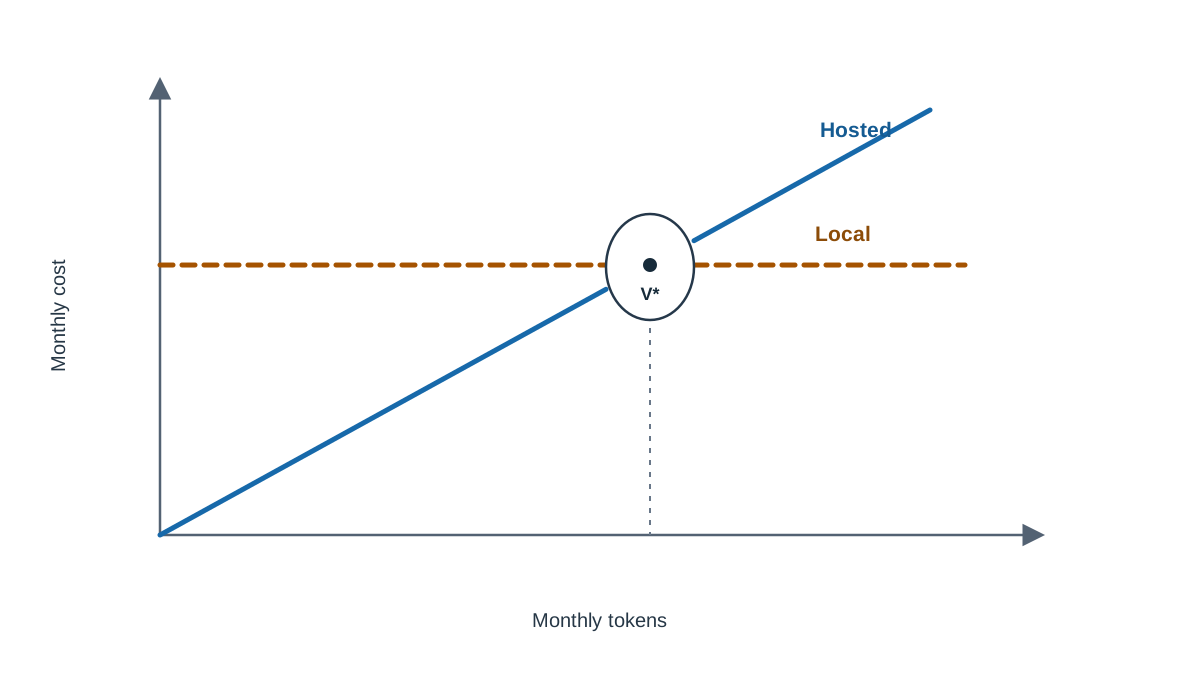
Start with the hosted side. If V is tokens per month and p is dollars per million tokens, monthly hosted cost is:
C_hosted = (V / 1,000,000) × p
Linear in volume. No floor. Nothing to amortize.
Now the local side. The one-time cost H spreads across the horizon, and the recurring cost M applies every month:
C_local = H / T + M
Flat in volume. The H / T term is the amortized truth of hardware depreciation — not a fiction, just a cost you paid up front and are now spreading out.
Set them equal, because break-even is the volume where the two paths cost the same:
(V / 1,000,000) × p = H / T + M
Solve for V:
V* = (H / T + M) × 1,000,000 / p
Read the structure out loud, because it tells you everything:
- The numerator is your monthly local burden — amortized hardware plus operating cost.
- The denominator is how much each hosted token costs you.
V*is a rate, not a total: the monthly token volume at which the two paths cost the same over the stated horizon.
The asymmetry is now visible in algebra. Raise T and V* falls. Raise p and V* falls. Raise M and V* rises. Every argument about hosted versus local is really an argument about one of those three terms.
Knowledge check
Check your understanding
Answer this question before you continue.
Worked Example: One Workload, Two Verdicts
Let us run it with illustrative numbers. These are hypothetical planning figures, not current market prices, and they are horizon-dependent.
Assume a small team with a workstation-class GPU:
H= $2,500 (hardware plus setup)M= $150 per month (electricity plus a few hours of maintenance)T= 12 months
The monthly local burden is $2,500 / 12 + $150 ≈ $358 per month.
Now change only the comparison target.
| Comparison tier | p ($/M tokens) | V* (tokens/month) | Reading |
|---|---|---|---|
| Budget hosted tier | $0.50 | ~716 million | Local wins only at very high volume |
| Frontier tier | $13.00 | ~27.5 million | Local wins at moderate volume |
| Cheap open-weight endpoint | $0.10 | ~3.58 billion | Local effectively never wins in 12 months |
Same hardware. Same workload. Same horizon. Only the alternative changed, and the crossover moved by more than two orders of magnitude.
That is the second break-even, and it is why quoting a single number is misleading. The hardware did not get cheaper or more expensive. You just changed what you were comparing it against.
Common mistake: Comparing your hardware price against a frontier API bill, then concluding local wins. If your workload runs on an open-weight model, the honest comparison is the cheap open-weight endpoint — and that comparison usually kills the case.
Knowledge check
Check your understanding
Answer this question before you continue.
Utilization Is the Assumption That Breaks the Model
The flat local cost is only flat if the hardware is actually busy. Idle GPUs still draw power and still depreciate.
Here is the bridge the equation above hides. V is monthly token volume. Utilization is how much of the hardware's capacity that volume actually consumes. They are different quantities, and the model above quietly assumes utilization is high enough that capacity never binds.
To make utilization explicit, add one term. Let U be the fraction of the box's practical monthly capacity that your workload actually uses, and let C_max be the token volume the hardware can serve per month at full saturation. Then:
U = V / C_max
When U is high, your M estimate is roughly right: the box is earning its keep. When U is low, the same M is spread across fewer tokens, and effective cost per token rises. The clean way to capture that in the model is to treat M as a function of utilization — power draw and maintenance don't shrink just because the box is idle:
C_local_per_M = (H / T + M) × 1,000,000 / V
As V falls, cost per token rises without limit. This is the mirror image of hosted pricing: hosted has no floor, local has no ceiling.
Now run the sensitivity. Suppose the same box can serve C_max = 300 million tokens per month at full saturation, and your workload actually pushes V = 90 million tokens per month. That is U = 30%. The $358 monthly burden now spreads across 90 million tokens instead of 300 million, so effective local cost is roughly three times higher per token than at saturation. Plug that back into the break-even equation and V* — the hosted volume at which local stops winning — moves up by the same factor.
Duty cycle matters more than peak throughput. A box that runs at 30% average load during working hours costs roughly three times per token what the same box costs at full saturation. And workload type compounds it: long-context and retrieval-style workloads consume far more compute per token than short chat calls, which pushes effective local cost per token up and the break-even volume higher.
Tip: Instrument two weeks of real traffic and bucket tokens by hour before trusting any utilization figure you assumed. That single measurement replaces the assumption most likely to be wrong.
Knowledge check
Check your understanding
Answer this question before you continue.
The Costs That Never Appear on the Receipt
The most common beginner mistake is comparing hardware price against an API bill and calling it total cost of ownership. It is not.
Setup and hardening time belongs in H. Getting a runtime working, choosing quantization, tuning context length, and wiring monitoring is a one-time cost. It is real money even when nobody invoices it.
Ongoing maintenance belongs in M. Model updates, driver and security patches, monitoring, and troubleshooting. A few hours a month is a reasonable planning figure, not a worst case. Multiply those hours by a loaded labor rate and the number stops looking small.
Storage and bandwidth. Model weights are large, and keeping multiple versions multiplies that. Downloading them over a slow connection wastes time you cannot get back.
Opportunity cost. Hours spent maintaining inference infrastructure are hours not spent on the product the inference exists to serve.
Depreciation and replacement. Hardware has a useful life shorter than most planning horizons assume. H / T is not a fiction. It is the amortized truth.
When the Model Says Local, and When It Lies
Trust the arithmetic when volume is high and sustained, the workload genuinely runs on the local model, and the horizon is long enough for hardware to amortize.
Distrust it when volume is spiky, the workload needs a frontier model, or the box would sit idle most of the day.
Two traps are worth naming explicitly.
The sunk-cost trap. Once hardware is bought, teams route everything to it, including work that needed a stronger model. Quality degrades in places nobody is measuring. Sunk hardware is a reason to use the model more. It is a poor reason to use a worse model for work that needed a better one.
The private-API trap. A private tier on a hosted service is still someone else's servers. If the requirement is that data never leaves your infrastructure, cost is not the deciding variable.
The pattern that usually survives contact with reality is hybrid: local for high-volume, sensitive, or routine tasks; hosted for low-volume, high-reasoning tasks. Two break-evens, one architecture.
And be honest about scope. This model excludes latency, reliability, compliance, and vendor risk. Those are separate decisions with their own criteria.
What to Do Next
Do not start with a calculator. Start with three sentences: the horizon you are planning over, the exact hosted tier you would otherwise buy, and the utilization you expect. Write them down before you touch any numbers, because those three choices decide the answer.
Then solve for V*. Then re-run it twice — once with a pessimistic U that raises your effective M, and once with the frontier-tier price — and see whether your answer survives. If it flips, you did not have a break-even point. You had a preference with arithmetic attached.
The one measurement worth doing this week: instrument two weeks of real token traffic and bucket it by hour. That replaces the assumption most likely to be wrong with data you actually own.
Knowledge check
Final check
Finish the article by checking the ideas you just learned.
References
Want a more structured LLMOps path?
Use the LLMOps Practical Starter Bundle to connect RAG, evaluation, observability, and production patterns.
Large Language Models Starter Pack
A 12-chapter guide connecting LLM fundamentals with prompting, RAG, agents, tool calling, evaluation, security, and application engineering.
- 227-page Illustrated PDF edition
- 12 guided LLM engineering chapters
- Visual concept diagrams
- Self-assessment quizzes
- Bonus deep-dive sections
- Prompt design, structured output, context windows & RAG pipelines
- Agents, tool calling, prompt injection, evaluation & application lifecycles
Coming soon


