How a Training Loss Produces Gradients

You watch the loss number fall on a training chart. Something inside the model changed, but the chart never tells you what. The loss is a single number, and a single number cannot point anywhere. The direction has to come from somewhere else.

That "somewhere else" is the gradient. Here is the whole chain in one sentence: the loss measures how wrong the model is, the gradient measures how sensitive that wrongness is to each parameter, and the optimizer uses that sensitivity to nudge every parameter in a direction that should reduce the error. One scalar in, one direction out.

We will carry one toy example end to end: one weight, one input, one target, one gradient, one update. By the end you will be able to compute all of it by hand.

What the Loss Actually Hands You

You already know that language-model training minimizes a next-token cross-entropy loss. The part worth pausing on is what that loss is at the moment of the backward pass: a scalar. A single floating-point number summarizing the error across an entire batch of predictions.

A scalar has magnitude but no direction. It can tell you how wrong the model was. It cannot tell you which way to move any of the millions of parameters that produced it.

So we ask a different question, one parameter at a time: if I nudge this weight slightly, how much does the loss move? That sensitivity is the derivative. Stack the derivative for every parameter into one vector and you have the gradient — a direction in a very high-dimensional space.

Picture the loss as a curve over a single parameter. The current weight sits at one point on that curve. The slope at that point is the gradient. It tells you which way is uphill. To go downhill, you walk the other way.

Notation and Assumptions Before Any Math

Before the arithmetic, define the symbols:

Symbol	Meaning
$\theta$	the full set of model parameters
$w$	a single weight, used for the toy case
$x$	an input
$\hat{y}$	the model's prediction
$y$	the target
$L$	the loss, a scalar
$\eta$	the learning rate, a step-size dial
$\nabla L$	the gradient, the vector of partial derivatives of $L$

Three assumptions make the rest of this work.

The loss is differentiable with respect to the parameters. This is a large part of why cross-entropy and mean squared error are so common: their derivatives are clean and cheap to compute. Some exotic losses have awkward or undefined gradients near decision boundaries, which makes training harder to stabilize.

We can compute the gradient for every parameter. That is what backpropagation delivers — an efficient way to get the derivative of the loss with respect to each weight without computing them one by one.

The gradient is a local linear approximation. It is accurate for small steps. It says nothing reliable about a jump across the whole curve.

When these assumptions fail, training misbehaves in recognizable ways: non-differentiable losses stall, vanishing gradients shrink to nothing in deep stacks, exploding gradients blow up, and steps so large that the linear approximation is meaningless send the loss upward instead of down.

From One Prediction to One Gradient

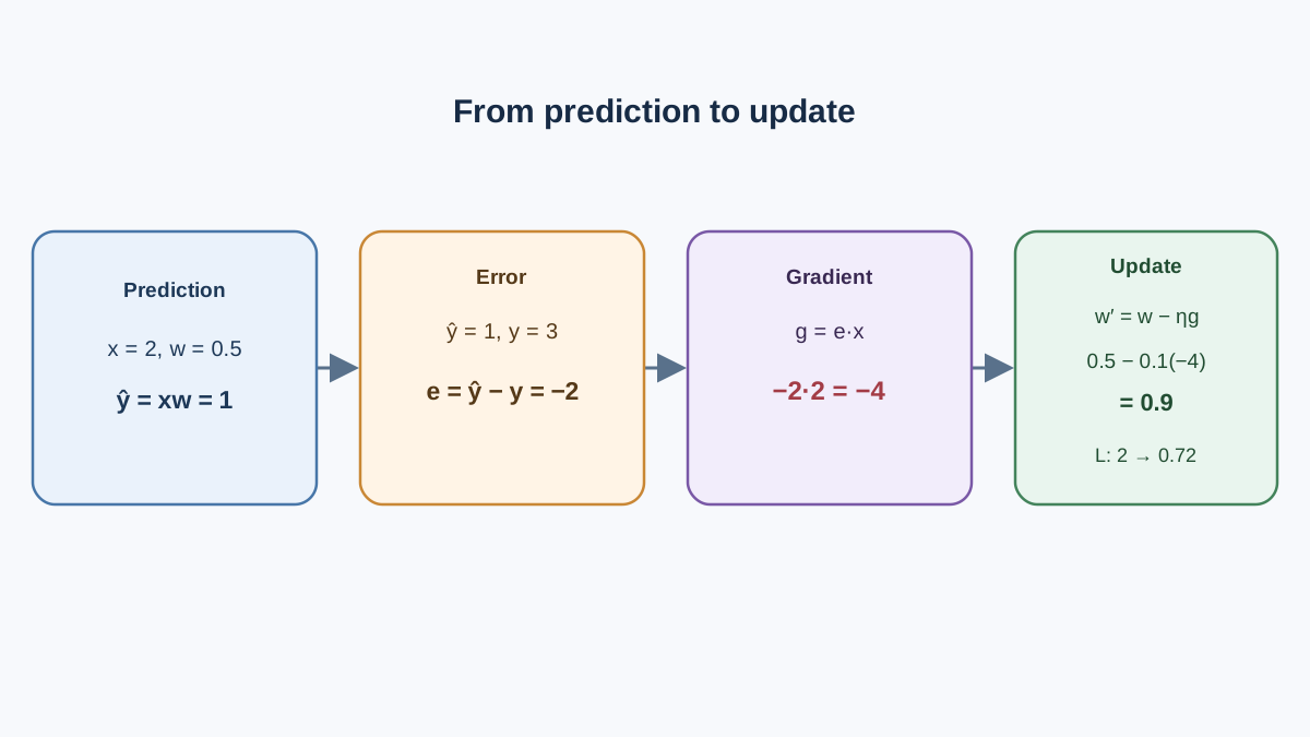
Take the smallest possible case. One input $x$, one weight $w$, prediction $\hat{y} = w \cdot x$, and squared-error loss:

$L = \tfrac{1}{2}(\hat{y} - y)^2$

The $\tfrac{1}{2}$ is there purely to cancel the exponent when we differentiate. Now derive the gradient in three steps.

First, how does the loss change with the prediction?

$\frac{\partial L}{\partial \hat{y}} = (\hat{y} - y)$

That is just the error. Positive error means the prediction was too high; negative means too low.

Second, how does the prediction change with the weight?

$\frac{\partial \hat{y}}{\partial w} = x$

Third, chain them together:

$\frac{\partial L}{\partial w} = (\hat{y} - y) \cdot x$

Read the two factors. The error term sets the magnitude and the sign. The input term says how much this weight mattered for this example — a large input amplifies the weight's influence, so its gradient is larger.

Now plug in numbers. Let $x = 2$, $w = 0.5$, $y = 3$.

$\hat{y} = 0.5 \cdot 2 = 1$

$\text{error} = 1 - 3 = -2$

$\frac{\partial L}{\partial w} = (-2) \cdot 2 = -4$

The gradient is $-4$. The negative sign means: to reduce the loss, increase this weight. And notice the general pattern — gradient magnitude scales with error size. Large early errors produce large early steps. That is not a bug; it is the mechanism doing its job.

Turning the Gradient Into a Parameter Update

The gradient tells you the direction of steepest increase. You want decrease, so you step the other way. The gradient descent update rule is:

$w \leftarrow w - \eta \cdot \frac{\partial L}{\partial w}$

With $\eta = 0.1$ and our gradient of $-4$:

$w \leftarrow 0.5 - 0.1 \cdot (-4) = 0.5 + 0.4 = 0.9$

Recompute the loss at the new weight. The prediction becomes $0.9 \cdot 2 = 1.8$, the error becomes $-1.2$, and the loss drops from $2$ to $0.72$. One step, and the model is measurably less wrong.

The minus sign is the whole trick. The gradient points uphill; you walk downhill.

The learning rate $\eta$ is the step-size dial. Too small and training crawls, burning compute on microscopic corrections. Too large and you overshoot the minimum — or diverge entirely, with the loss climbing every step.

Common mistake: Treating the learning rate as a minor knob. It is the single most consequential hyperparameter in this update. The gradient supplies the direction; the learning rate decides whether you arrive or fly past.

Real optimizers like Adam modify this rule with momentum and per-parameter scaling, so different weights get different effective step sizes. But the gradient still supplies the direction. Everything else is a smarter way of choosing how far to walk.

Why the Loss Does Not Fall Every Step

Here is the assumption beginners trip over: a correctly computed gradient does not guarantee a smaller loss on the next step.

Gradient descent is a local linear approximation. If the step is large enough, you land on a part of the curve where the slope was different from what the gradient predicted. The loss can rise even though the gradient was perfect.

Mini-batch gradients add a second source of noise. Each batch is a sample, so its gradient is an estimate of the true gradient, not the true gradient itself. Individual steps can move the loss the wrong way while the trend over many steps still improves.

There is also a practical failure mode worth naming: gradient accumulation. When you accumulate gradients over several steps before updating, the size of the resulting update depends on how those gradients are combined. If they are summed, the update is larger; if they are averaged, the update stays comparable to a single step. Push the summed version too far and the update overshoots — the loss can explode, and the gradients can go to infinity. That is the same overshoot problem as a too-large learning rate, arriving through a different door.

Practical read: Judge training by the trend across many steps, not by any single step's loss value. One bad step is noise. A rising trend is a signal.

What This Mechanics Does Not Promise

A small training loss means one thing: the model assigns high probability to the training targets. That is the entire claim.

It does not promise truthful outputs. It does not promise useful, well-calibrated, or safe ones. Those are separate questions about the data, the objective, and how you evaluate the result.

Lower loss on the training distribution can coexist with worse behavior on inputs that distribution does not cover. The same gradient machinery that teaches a model to predict fluently also teaches it to predict confidently — including when it is fabricating. Fluency and fabrication are both learned from the same signal.

This is the boundary I want you to hold onto: optimization mechanics describe how parameters move. They say nothing about whether the resulting behavior is good. A falling loss curve is evidence about optimization, not a certificate of quality.

A Tiny Check You Can Run Yourself

Do not take the derivation on faith. Verify it. The whole example fits in a few lines:

w, x, y, lr = 0.5, 2.0, 3.0, 0.1

for step in range(5):
    pred = w * x
    loss = 0.5 * (pred - y) ** 2
    grad = (pred - y) * x
    print(f"step {step}: w={w:.3f} loss={loss:.3f} grad={grad:.3f}")
    w -= lr * grad

Run it and watch the loss fall while the gradient shrinks toward zero as the weight approaches the value that makes the prediction match the target.

Then change one thing at a time. Set lr = 0.01 and watch the crawl. Set lr = 1.5 and watch it overshoot and oscillate. Change y and watch the gradient sign flip. Each change connects arithmetic to behavior, and the behavior is the point.

Where This Leaves You

The chain is short and it never changes: a scalar loss, differentiated with respect to each parameter, produces a gradient; the gradient supplies direction; the learning rate supplies distance; the optimizer applies the step. When training misbehaves, check the step size and the gradient magnitude before you blame the architecture. Those two numbers explain most instability.

The next concept in this path is how optimizers like Adam reshape this basic update — adding momentum and per-parameter scaling so the same gradient produces a smarter step. The gradient still does the pointing. The optimizer just learns how far to trust it.