
How Fine-Tuning Data Weights Change the Training Objective
You duplicate a handful of "good" examples to push the model toward a behavior. You retrain. The behavior barely moves — or it moves somewhere you did not…

Key topics
You duplicate a handful of "good" examples to push the model toward a behavior. You retrain. The behavior barely moves — or it moves somewhere you did not intend. The dataset got bigger, so why did the signal not get louder?
Because the training objective is not a pile of examples. It is a weighted average, and an average is a budget. Every example you add spends part of that budget and takes it away from every other example. This tutorial writes that budget down, computes it on a toy dataset, and then draws a hard line between moving the objective and improving the model.
If you have not yet reviewed what fine-tuning changes and when prompting or retrieval is the safer first move, the short version is enough here: fine-tuning continues training on a small targeted dataset, adjusting existing weights rather than starting from scratch. The question this article asks is narrower — what does the composition of that dataset do to the number being minimized?
Why "More Examples" Is Not a Weight
The common belief is proportional: add more examples of a behavior, get more of that behavior. Grant the narrow case where this holds. In a balanced dataset with no duplication, adding examples of a behavior does increase that behavior's share of the signal — roughly in proportion to how many you added.
The hidden mechanism is that the optimizer minimizes an average loss over the batch. Each example's influence is its share of the total, not its count in isolation. Double one group's size and you have changed every other group's share, even though you never touched those examples.
Think of the objective as a fixed pie of attention. The pie does not grow when you add examples. The slices get thinner. Add a hundred examples of one behavior and you have not added a hundred units of influence — you have diluted everything else to make room.
This is the model I want you to hold: weights redistribute emphasis; they do not create information. A weight is a multiplier on a signal that already exists in your data. If the signal is not there, no multiplier will conjure it.
One scope note before the notation. We are modeling the training objective — the number the optimizer minimizes. We are not predicting deployment behavior. Those are different claims, and conflating them is the most common mistake in this whole area.
Knowledge check
Check your understanding
Answer this question before you continue.
Notation: Writing the Objective Down
Let the dataset have examples. Each example has an input, a target output, and a per-example loss measuring how wrong the model is on that example.
The unweighted objective is the plain average:
That is what "minimize the loss" means in code. Nothing exotic.
Now group the examples. Suppose each example belongs to exactly one group , and group has examples with average loss . Assign each group a weight — a multiplier applied to every example in that group. The weighted objective is:
The division by is the part people skip, and it matters. Without normalization, scaling every weight up by ten changes the gradient magnitude, not the relative emphasis. That is a learning-rate question, not a composition question. Normalizing keeps the weights a statement about relative emphasis, so the objective stays comparable across weighting schemes.
Two assumptions are baked in, and I want them visible. First, this is a simplified objective: real fine-tuning adds optimizer dynamics, batching, and learning-rate schedules that we are deliberately holding fixed. Second, the groups must be a meaningful partition — every example in exactly one group, and the groups must correspond to something you actually care about. If the groups are arbitrary, the weights encode a fiction.
Knowledge check
Check your understanding
Answer this question before you continue.
A Toy Dataset With Uneven Groups
Let us build something small enough to check by hand. Three groups, deliberately imbalanced:
| Group | Examples | Average loss |
|---|---|---|
| Routine formatting | 90 | 0.20 |
| Edge-case handling | 8 | 0.60 |
| Refusal behavior | 2 | 0.80 |
The unweighted average loss is:
Look at where that number comes from. Routine formatting contributes of the total loss. Edge cases contribute about 20%. Refusals contribute about 7%.
Picture a stacked bar: one wide block of formatting, a thin sliver of edge cases, a thinner sliver of refusals. The big group owns the number. It owns it because of count, not because it is the hardest or the most important.
Here is the trap. The group with the most examples is not necessarily the group with the highest loss — refusals have the highest per-example loss here — and neither is necessarily the group you care about. The objective does not know what you care about. It only knows counts and losses.
Knowledge check
Check your understanding
Answer this question before you continue.
Worked Example: Moving the Weights
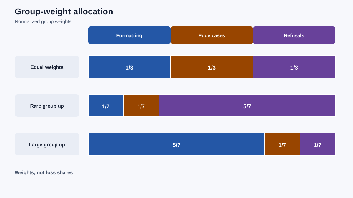
Start with equal weights, , so . Each group gets :
Wait — that does not match the unweighted average of 0.244. This is the first real lesson, and it is worth pausing on.
Equal group weights are not the same as equal example weights. The unweighted average weights each example equally, which means the 90-example group dominates. Equal group weights weight each group equally, which means the 2-example refusal group now carries the same influence as the 90-example formatting group. Same dataset, two different objectives. The composition of the dataset and the weighting scheme are separate decisions.
Now upweight the rare group. Set , so :
Refusals now contribute about 83% of the objective. The optimizer is now most willing to trade error on formatting to reduce error on refusals.
Flip it. Upweight the large group instead, , :
| Weighting | Formatting share | Edge-case share | Refusal share | |
|---|---|---|---|---|
| Equal examples | 74% | 20% | 7% | 0.244 |
| Equal groups | 33% | 33% | 33% | 0.533 |
| Rare group up | 4% | 13% | 83% | 0.686 |
| Large group up | 42% | 25% | 33% | 0.343 |
Read the table as a statement about which errors the optimizer is most willing to trade. Upweighting a group does not add information the dataset never contained. It changes the exchange rate between one kind of error and another.
Warning: Weight is a multiplier, not a filter. If the rare group's examples are inconsistent or mislabeled, upweighting them amplifies the inconsistency. You have made the noise louder, not the signal.
Knowledge check
Check your understanding
Answer this question before you continue.
What the Weighted Objective Does Not Tell You
A lower weighted training loss is a statement about the examples you supplied. It is not a statement about the distribution you care about.
The gap is structural, not a matter of effort. The objective is computed on observed examples. Generalization is a claim about unobserved ones, and the objective contains no term for them. You can drive toward zero and learn nothing about whether the model handles a case that was never in the dataset.
The assumption that breaks is the one from the notation section: that your groups are a meaningful partition of the behavior you want. If the groups are arbitrary, or if examples leak across them, the weights encode a fiction. You will get a clean number for a question nobody asked.
The common mistake is treating a reweighting experiment as a validated improvement. The objective moved. Whether the model got better is a separate measurement, on data the weighting never touched.
What would actually provide evidence? Held-out examples drawn from the target distribution, evaluated after training, with the weighting scheme fixed in advance. Fixing it in advance matters — if you try five weightings and report the best held-out score, you have quietly turned your test set into a training signal.
Note: Say what is known, what is inferred, and what should not be assumed. Known: the arithmetic above. Inferred: that the weighting will shift behavior in the direction you want. Not assumed: that it improves performance on cases you have not measured.
When Reweighting Helps and When It Misleads
Reweighting helps when three conditions hold together: you have a genuine coverage problem, the rare group is well-labeled, and you can measure the target behavior on held-out data. Miss any one and you are guessing with extra steps.
It misleads when you use weights to compensate for missing data, to paper over inconsistent labels, or to chase a metric you cannot evaluate. Weights redistribute emphasis. They do not create content.
Contrast with adjacent interventions. If the problem is missing knowledge, retrieval or more data addresses it directly. If the problem is instruction-following, prompting may be the cheaper first move. Reach for weights only when the data is present, correct, and under-emphasized.
The rule I would use: change one weighting variable at a time, record the objective value, and evaluate on data the weighting never touched. And watch the cost side — aggressive weighting can starve the majority group and degrade behavior you were not measuring.
Before you touch a weight, write down two things: the objective you are actually minimizing, and the held-out measurement you will use to judge the result. If you cannot name both, the reweighting is a guess dressed as a method.
The next practical step is small: take your own dataset, split it into groups, and compute under two or three weighting schemes by hand. Record the numbers before you train anything. Then go measure what the model actually does on cases the weights never saw — because that measurement, not the objective value, is what tells you whether the change was worth making.
Knowledge check
Final check
Finish the article by checking the ideas you just learned.
References
Want a more structured LLMOps path?
Use the LLMOps Practical Starter Bundle to connect RAG, evaluation, observability, and production patterns.
Large Language Models Starter Pack
A 12-chapter guide connecting LLM fundamentals with prompting, RAG, agents, tool calling, evaluation, security, and application engineering.
- 227-page Illustrated PDF edition
- 12 guided LLM engineering chapters
- Visual concept diagrams
- Self-assessment quizzes
- Bonus deep-dive sections
- Prompt design, structured output, context windows & RAG pipelines
- Agents, tool calling, prompt injection, evaluation & application lifecycles
Coming soon


