
Calculate a Gradient-Based Parameter Update
You can recite "gradient descent" and still freeze when someone hands you a loss, a gradient, and a learning rate. That freeze is not a math problem. It is…

Key topics
You can recite "gradient descent" and still freeze when someone hands you a loss, a gradient, and a learning rate. That freeze is not a math problem. It is a missing mental model: the update rule is a signed step on a curve, not an incantation. By the end of this article, you will hand-compute one update, predict whether the next loss falls, and know exactly which assumption would break your prediction.
We will keep the example tiny on purpose — one parameter, one data point — so the arithmetic never hides behind notation. If you have not yet seen how a training loss turns into a gradient, that is the prerequisite; here we pick up right after the gradient exists and push it through an update.
What You Need Before the Arithmetic
Two assumptions carry this entire article. First, the loss is differentiable at the point we evaluate it — the curve has a well-defined slope there. Second, we can compute or estimate that slope. If either fails, the update rule below does not apply, and no amount of tuning will rescue it.
Fix the notation once, and the rest reads as bookkeeping:
| Symbol | Meaning |
|---|---|
| the parameter we are adjusting (a weight, in a real model) | |
| the loss as a function of that parameter | |
| the gradient — the slope of the loss with respect to | |
| the learning rate, a positive scalar | |
| the iteration index |
One boundary up front, because it is the most common confusion: everything here is optimization mechanics. A smaller loss is a statement about a number. It is not a promise that the trained model will be truthful, useful, or well-calibrated. Those are separate claims, and we will return to that gap at the end.
The Update Rule, Read Symbol by Symbol
Start from the goal, not the formula. We want a small change in that makes smaller.
Near the current point, the loss behaves almost like a straight line. That is the first-order approximation:
To reduce , we want the change term to be negative. The gradient points in the direction of steepest increase — uphill. So we step the other way. Set with , and the change becomes , which is negative whenever the gradient is nonzero. The loss drops.
That gives the plain gradient-descent update:
Read it in words: new parameter equals old parameter minus a scaled copy of the slope. The minus sign is not a convention to memorize. It is the direction that makes the linear approximation decrease, and it falls straight out of the goal.
What does multiply? The step size, not the direction. The gradient decides which way to move; decides how far. And notice the honesty in the approximation: the straight-line model is only valid locally. Take too large a step and you leave the region where the line still resembles the curve — which is exactly why cannot be arbitrarily large.
Knowledge check
Check your understanding
Answer this question before you continue.
A Toy Loss You Can Differentiate by Hand
Pick the simplest loss with a clean derivative:
The target is , where the loss is zero. Differentiate:
Start at . The gradient there is . Two things to read from that number. The sign is negative, which means the loss decreases as increases — downhill is to the right. The magnitude, 6, says the curve is steep at this point, so a given step size buys a large move.
The loss at the start: . Hold onto that 9. It is your before-number.
Knowledge check
Check your understanding
Answer this question before you continue.
Run One Update and Check the Loss
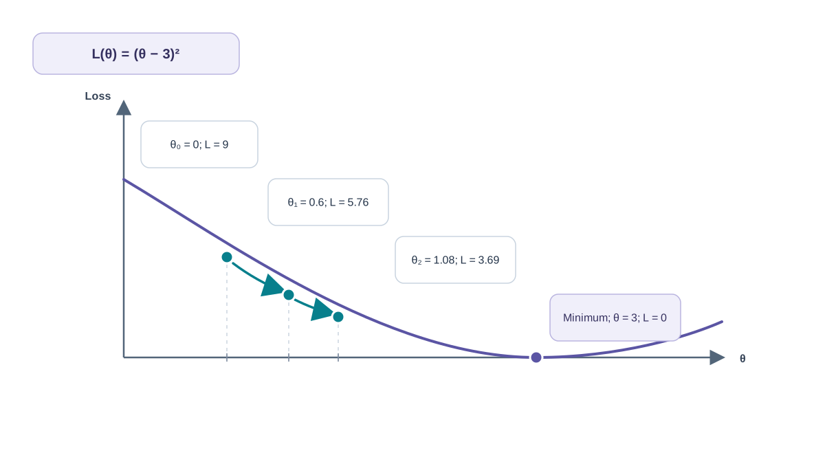
Choose . Apply the rule with the numbers visible:
The negative gradient pushed to the right, from 0 to 0.6 — exactly the direction the sign predicted. Now check whether the loss actually fell. . It dropped from 9 to 5.76 — a real decrease, not a hoped-for one.
Run a second iteration to see the pattern rather than a single lucky step. The gradient at is . So:
And . Down again. The parameter is marching toward 3, and the steps are shrinking because the gradient shrinks as we approach the bottom.
Note: With this loss and this , the parameter approaches the target smoothly without overshooting. That is a property of this example — a simple convex bowl and a modest step size — not a universal guarantee. Change the loss or the learning rate and the behavior changes.
Knowledge check
Check your understanding
Answer this question before you continue.
What the Learning Rate Actually Controls
The learning rate is the one knob you can reason about directly, so let us vary it on the same loss and watch the consequences.
Too small. Set . From , the first step moves to . The loss barely budges. You will still converge, but you will spend thousands of iterations crawling toward a target you could have reached in a handful. Slow, safe, wasteful.
Too large. Set . The first step jumps from 0 to 6 — past the target at 3, all the way to the other side. The next gradient is , so the step goes back to . You are now oscillating between 0 and 6 forever, never landing. Push past 1.0 and the loss grows each step: divergence.
The tradeoff in one sentence: trades speed against stability, and the safe range depends on the curvature of the loss. A sharply curved loss tolerates a smaller step than a gentle one.
Common mistake: When a real training run oscillates or the loss explodes, the instinct is to blame the data or the architecture. Check the step size first. A learning rate that is too high produces exactly this signature, and it is the cheapest thing to test.
Knowledge check
Check your understanding
Answer this question before you continue.
From One Parameter to Real Optimizers
The skeleton you just used survives in every production optimizer. Compute a gradient estimate, scale it, subtract it from the parameters. What changes is how the scaling is done.
Plain stochastic gradient descent (SGD) uses one global for every parameter. Momentum adds a running average of past gradients, which smooths the direction and damps oscillation across narrow valleys. Adam-style methods go further: they track a running average of the gradient (the first moment) and of the squared gradient (the second moment), then divide the step by the square root of that second moment. The effect is a per-parameter step size learned from each parameter's own gradient history.
The Adam update has this shape:
Here and are bias-corrected estimates of the first and second moments, and is a tiny constant that exists for one reason: to avoid dividing by zero when the second moment is near zero.
What changes: the per-parameter step size is now learned from gradient history instead of fixed. What does not change: the shared update framework — compute a direction, scale it, subtract it from the parameters. The Adam step is not simply the negative of the current gradient, though. It is a history-scaled direction, so the analogy to the toy example holds at the level of the skeleton, not at the level of the exact vector you subtract.
Where This Model Breaks
The mechanics are clean, which makes them easy to over-trust. Four places where the clean story stops being true:
- The linear approximation is local. Large steps invalidate the reasoning that produced the update. The direction was justified by a straight line that no longer fits the curve.
- A small training loss is not a promise about behavior. You optimized a number. Whether the model is truthful, useful, or well-calibrated is a different question with different evidence.
- Gradient estimates from mini-batches are noisy. A single update can move the loss the wrong way even when the rule is applied correctly, because the gradient you used was an estimate, not the true slope.
- Non-convex losses mean you find a lower point, not the lowest point. Real neural networks do not have a single bowl. The update descends; it does not guarantee arrival at a global minimum.
Warning: Do not read a falling loss curve as proof that the model is getting better at the thing you care about. It is proof that the optimizer is doing its job on the objective you gave it.
Your Next Move
Here is the drill. Take the same loss, , and change three things: the starting point, the target, and . Before you compute each update, predict whether the next loss will fall, and by roughly how much. Then run the arithmetic and check yourself. The prediction is the skill; the arithmetic is just the receipt.
When a real training run misbehaves, use this order: check the step size, then check gradient noise, then look at the architecture. The first two are cheap and explain most of what you will see.
The next layer of the same mechanism is how optimizers interact with learning-rate schedules and batch size — because both quietly change the effective step size you just learned to reason about.
Knowledge check
Final check
Finish the article by checking the ideas you just learned.
References
Want a more structured LLMOps path?
Use the LLMOps Practical Starter Bundle to connect RAG, evaluation, observability, and production patterns.
Large Language Models Starter Pack
A 12-chapter guide connecting LLM fundamentals with prompting, RAG, agents, tool calling, evaluation, security, and application engineering.
- 227-page Illustrated PDF edition
- 12 guided LLM engineering chapters
- Visual concept diagrams
- Self-assessment quizzes
- Bonus deep-dive sections
- Prompt design, structured output, context windows & RAG pipelines
- Agents, tool calling, prompt injection, evaluation & application lifecycles
Coming soon


