
Model the Cost and Stale-State Risk of Agent Memory
A team sets memory to refresh every six hours to save money. Four hours later, an agent quotes a price, policy, or preference that has already changed. The…

Key topics
A team sets memory to refresh every six hours to save money. Four hours later, an agent quotes a price, policy, or preference that has already changed. The instinct is to blame the model. The real failure is an unpriced tradeoff.
If you have audited agent memory by hand, you know how to spot a stale record after the fact. This article is about the question that comes next: how often should you refresh stored state in the first place, and how do you justify that choice with numbers instead of vibes? The answer is not "as often as possible." It is a small model with three cost terms you can actually compare.
Note: This is a back-of-the-envelope model. Its job is to expose your assumptions and make them arguable, not to hand you a universal refresh schedule.
Why "Refresh More Often" Is Not a Strategy
The default belief is that fresher memory is strictly better, so you should refresh as often as your budget allows. There is a narrow case where that is true: when refresh is nearly free and stale actions are catastrophic. Outside that case, the belief hides two constraints.
Every refresh costs money. Every stale read carries some probability of a wrong action with a real impact. Treating freshness as a free good ignores the first constraint. Treating cost as the only real constraint ignores the second. The decision is a tradeoff between two measurable costs and one probabilistic risk.
Name the three terms now, because everything below builds on them:
- Retrieval cost — what you pay every time the agent reads memory.
- Refresh cost — what you pay every time you rebuild or re-fetch stored state.
- Stale loss — the expected cost of acting on information that has gone out of date.
Auditing tells you which records are stale. This model tells you how often to prevent staleness in the first place. It is the scheduling layer on top of the audit work you already know.
The Variables You Need Before You Can Decide
Define notation before using it, and attach each symbol to the mechanism it represents.
| Symbol | Meaning | Mechanism it represents |
|---|---|---|
| τ | Horizon | The fixed window you are planning over, such as 24 hours |
| Δ | Refresh interval | How often you rebuild or re-fetch stored state |
| N | Request count | How many agent requests occur during τ |
| c_r | Retrieval cost | Cost of reading memory once, per request |
| c_u | Refresh cost | Cost of one refresh |
| p_s(Δ) | Stale-action probability | Assumed per-request chance the agent acts on outdated state |
| L | Impact | Cost of one stale action |
A few of these deserve a sentence of care.
Horizon τ is the window you plan over. Everything is measured inside it. Pick something concrete — a day, a week, a billing period.
Refresh interval Δ is the lever you are actually choosing. Smaller Δ means fresher memory and more refreshes. This is the variable the whole model exists to set.
Request count N is how many agent requests happen during τ. Assume requests are distributed across the horizon rather than clustered at the start. If they are bursty, the model still works, but the timing of refreshes matters more than their count.
Stale-action probability p_s(Δ) is the one you have to supply yourself. It is an assumed per-request probability, not a universal law. It depends on how fast the underlying data changes and how much of that change the agent actually reads. A memory of a user's preferred language barely drifts. A memory of a live price can drift every minute.
Impact L must be in the same units as the other costs, so the terms can be added. If c_r and c_u are in dollars, L is in dollars. If they are in latency, L is in latency. Mixing units is the fastest way to produce a confident, wrong answer.
Knowledge check
Check your understanding
Answer this question before you continue.
Deriving the Three Cost Terms
Derive each term separately, then add them. That way you can see which ones move with Δ and which ones do not.
Retrieval cost. Every request reads memory, regardless of how fresh it is:
Notice what this term does not contain: Δ. Retrieval cost is the same whether you refresh hourly or weekly. That fact will matter in the worked example.
Refresh cost. If you refresh once every Δ over a horizon τ, the number of refreshes is roughly τ/Δ:
For a finite horizon, use instead of τ/Δ, and exclude an initial refresh if the state starts fresh. The ceiling matters at the boundary: if τ = 24 hours and Δ = 5 hours, you cannot fit four refreshes cleanly, so you round up to five. Ignoring the ceiling undercounts refresh cost slightly, which is exactly the kind of error that makes a cheap schedule look cheaper than it is.
Stale loss. This is an expected value, not a guarantee. It is the average loss if the same scenario ran many times:
Total. Sum the three terms:
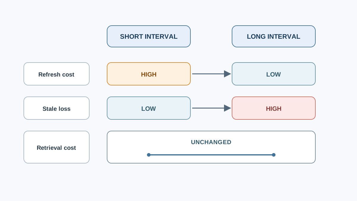
Only two of the three terms move with Δ, and they move in opposite directions. Smaller Δ raises refresh cost and lowers stale loss. That opposition is the entire tradeoff, and it is why "refresh more often" cannot be a strategy on its own.
Common mistake: Assuming p_s is constant across the horizon. If the underlying data changes in bursts — a pricing update at midnight, a policy change on Mondays — then p_s is higher right after the burst and lower later. A single average hides that structure.
Knowledge check
Check your understanding
Answer this question before you continue.
Worked Example: 24 Hours, Two Refresh Schedules
Run the numbers end to end so the model produces a comparable answer instead of an abstract inequality.
Setup: τ = 24 hours, N = 240 requests, c_r = $0.002, c_u = $0.05, L = $2.
Schedule A, Δ = 1 hour. Refreshes: 24, costing 24 × $0.05 = $1.20. With an assumed p_s = 0.005, stale loss is 240 × 0.005 × $2 = $2.40. Retrieval cost is 240 × $0.002 = $0.48. Illustrative total: $4.08.
Schedule B, Δ = 6 hours. Refreshes: 4, costing 4 × $0.05 = $0.20. With an assumed p_s = 0.03, stale loss is 240 × 0.03 × $2 = $14.40. Retrieval cost is still $0.48. Illustrative total: $15.08.
| Term | Δ = 1 hour | Δ = 6 hours |
|---|---|---|
| Retrieval | $0.48 | $0.48 |
| Refresh | $1.20 | $0.20 |
| Stale loss | $2.40 | $14.40 |
| Total | $4.08 | $15.08 |
The key observation: retrieval cost is identical in both cases, so it cancels out of the comparison. The decision is driven entirely by refresh cost versus stale loss. The cheaper schedule loses on total cost because the stale-loss term dominates.
Where does the ranking reverse? Solve for the L at which the two totals are equal. Schedule A's advantage is $1.00 in refresh cost ($1.20 − $0.20). Schedule B's disadvantage is its extra stale loss, which is . Setting gives L ≈ $0.17. Below roughly 17 cents per stale action, the six-hour schedule wins. Above it, the hourly schedule wins. That crossover is the whole decision, compressed into one number.
Knowledge check
Check your understanding
Answer this question before you continue.
Sensitivity: When the Answer Flips
The crossover above is conditional on the assumptions. Vary them and watch the conclusion move.
Vary L. If a stale action costs $0.10 instead of $2, the stale-loss term shrinks to $0.72 for Schedule B and $0.12 for Schedule A. Now the six-hour schedule totals $1.40 against $1.80 for the hourly one. The cheap schedule wins. Impact, not frequency, often decides the answer.
Vary p_s. If the underlying data barely changes, p_s stays low even at Δ = 6 hours. Suppose p_s = 0.002 at six hours: stale loss is $0.96, and the six-hour total is $1.64 versus $1.44 for hourly — close enough that the extra freshness is nearly free. Frequent refreshes become waste when the data is stable.
Vary c_u. If refresh is expensive — say a full re-embedding pass at $0.50 — the hourly schedule's refresh cost jumps to $12.00, and the tradeoff tightens sharply. Now the six-hour schedule wins even at L = $2: its total is $16.88 ($0.48 retrieval + $2.00 refresh + $14.40 stale loss), compared with $14.88 for the hourly schedule ($0.48 retrieval + $12.00 refresh + $2.40 stale loss). Higher refresh cost pushes the crossover point upward, making longer intervals more attractive.
The decision rule that falls out:
- Refresh more often when L is high or data changes fast.
- Refresh less often when refresh is expensive and stale actions are cheap and recoverable.
Warning: It is easy to tune p_s until it justifies the schedule you already wanted. The model exposes assumptions; it does not validate them. If your p_s estimate is a guess, say so, and run the sensitivity check before committing.
Knowledge check
Check your understanding
Answer this question before you continue.
What the Model Does Not Capture
Set honest boundaries so you do not over-trust a toy model.
p_s(Δ) is assumed, not measured. In practice you estimate it from logs, incident reports, or a small experiment. It may not be constant across the horizon, and it may not be independent across requests.
The model treats stale actions as independent. Real systems can cascade. One bad action seeds the next, and the error compounds rather than staying a one-off loss. When that risk is real, L is not a constant — it grows with each stale read.
It ignores latency, partial refreshes, and per-record freshness. Some memory entries change hourly; others change yearly. A single uniform Δ is a simplification.
It assumes one Δ for everything. Real systems often mix schedules: cheap high-churn records refreshed often, stable records refreshed rarely. That is a refinement, not a contradiction — you can run the model per record class and sum the results.
It prices staleness but does not detect it. Detection still needs provenance and freshness checks. This model tells you how much staleness costs; it does not tell you when a specific record has gone stale.
Your Next Move
Write down τ, N, c_r, c_u, L, and your best guess at p_s(Δ). Compute the three terms for two candidate intervals. See which one wins. Then run the sensitivity check — vary L and p_s by a factor of two in each direction and watch whether the ranking holds.
The point is not to produce a number you trust. The point is to make your assumptions visible and arguable, so the next time an agent acts on a price that changed four hours ago, you can point to the term that was underpriced instead of blaming the model.
Knowledge check
Final check
Finish the article by checking the ideas you just learned.
Want a more structured LLMOps path?
Use the LLMOps Practical Starter Bundle to connect RAG, evaluation, observability, and production patterns.
Large Language Models Starter Pack
A 12-chapter guide connecting LLM fundamentals with prompting, RAG, agents, tool calling, evaluation, security, and application engineering.
- 227-page Illustrated PDF edition
- 12 guided LLM engineering chapters
- Visual concept diagrams
- Self-assessment quizzes
- Bonus deep-dive sections
- Prompt design, structured output, context windows & RAG pipelines
- Agents, tool calling, prompt injection, evaluation & application lifecycles
Coming soon


