
Agent Loop Budgets: Model Iterations, Cost, and Stopping Risk
A loop that usually finishes in three steps can still spend most of its money on the runs that don't.

Key topics
A loop that usually finishes in three steps can still spend most of its money on the runs that don't.
You've probably seen this already. Your agent handles most requests in two or three iterations, so you budget for two or three iterations. Then one request spirals to the cap, and the bill for that single run is larger than the previous fifty combined. The average was fine. The average was also lying to you.
The cap is not a safety net you rarely touch. It is the shape of your worst case, and a single number — how likely the loop is to continue after any given step — decides how often you actually live there. In this article we build one small model of a bounded loop, derive what it says about expected cost and stopping risk, and then mark clearly where the model stops describing reality.
If you've already worked through how to set iteration limits and stopping rules, you know the qualitative version. Here we ask the quantitative follow-up: what does the cap actually cost you, and how often does it save you?
Why Averages Lie About Agent Loops
Three different questions hide inside the phrase "how much will this cost":
- Expected cost. On average, across many runs, what do I spend?
- Cap-hit probability. How often does a run fail to finish before running out of budget?
- Completion probability. How often does a run actually succeed?
These are not the same number, and optimizing one can quietly wreck another. A loop with a low average cost can still hit its cap constantly if the distribution is skewed. A loop that almost never hits its cap can still be expensive if each step is pricey. And a loop that hits the cap often might be fine — if hitting the cap is cheap and the user doesn't care about the truncated result.
The cap does two jobs at once, and they pull in opposite directions. It bounds spend — no run can exceed N steps. It also truncates work — any run that needed more than N steps gets cut off mid-task. Tighten the cap and you spend less but finish fewer tasks. Loosen it and you finish more but pay for the tail. There is no setting that maximizes both. The whole game is choosing where on that tradeoff you want to sit, and knowing what you're giving up.
Notation And Assumptions For A Toy Loop
Before any math, let's fix the symbols.
- p — the probability that the loop continues after any given step. Treated as constant across steps.
- N — the iteration cap. The maximum number of steps the loop is allowed to take.
- c — the cost of one step, in whatever unit you care about (dollars, tokens, seconds).
- K — the step at which the loop actually stops. This is a random variable; it depends on the run.
Three assumptions make the model tractable:
- p is constant. Every step has the same continuation probability, regardless of what happened before.
- Steps are independent. Whether step 3 continues tells you nothing about whether step 4 will.
- Per-step cost is uniform. Every step costs exactly c.
All three are false in production. That's fine. The point of a toy model is not to be true — it's to be transparent enough that you can see which assumption is doing the work, and then ask what changes when you relax it. We'll do exactly that in the last section.
Note: In a real loop, p is not a fixed property of the system. It's a summary of how often your agent, on a typical step, decides it isn't done yet. That number moves with the task, the model, the tools, and the prompt. Treat it as a range, not a constant.
Deriving Expected Iterations And Expected Cost
Here's the key move. Instead of asking "how many steps will this take?", ask "what's the probability the loop reaches step k?"
To reach step 2, the loop must continue after step 1. Probability: p.
To reach step 3, it must continue after step 1 and after step 2. Probability: p × p = p².
To reach step k, it must continue k − 1 times in a row:
Read that as a survival curve. It tells you what fraction of runs are still alive at each step. When p is small, the curve drops off a cliff. When p is close to 1, it stays high and flat — most runs survive deep into the loop.
The expected number of steps is the sum of these survival probabilities, from k = 1 up to the cap:
That's a geometric series. Without the cap, the sum would run to infinity and, for any p < 1, converge to 1 / (1 − p). The cap turns an infinite sum into a finite one — and that's the entire reason the cap exists as a cost control. It's not decoration. It's the term that makes the sum stop.
Expected cost is just expected steps times per-step cost:
Notice the asymmetry. Cost scales linearly in c — double the per-step price, double the bill. But it scales nonlinearly in p. As p approaches 1, the denominator collapses and expected cost explodes. That nonlinearity is why "it usually finishes fast" is such a dangerous intuition.
Worked example: p = 0.5, N = 6, c = $0.02
The naive guess: if the loop continues half the time, it should take about two steps. Let's check.
| Step k | P(reaches k) |
|---|---|
| 1 | 1.000 |
| 2 | 0.500 |
| 3 | 0.250 |
| 4 | 0.125 |
| 5 | 0.063 |
| 6 | 0.031 |
Sum of survival probabilities: 1 + 0.5 + 0.25 + 0.125 + 0.063 + 0.031 = 1.969 steps.
Expected cost: 1.969 × $0.02 = $0.039.
So the naive guess of two steps was almost exactly right. At p = 0.5, the geometric tail dies fast and the cap barely matters.
Knowledge check
Check your understanding
Answer this question before you continue.
The same numbers at p = 0.8
| Step k | P(reaches k) |
|---|---|
| 1 | 1.000 |
| 2 | 0.800 |
| 3 | 0.640 |
| 4 | 0.512 |
| 5 | 0.410 |
| 6 | 0.328 |
Sum: 1 + 0.8 + 0.64 + 0.512 + 0.410 + 0.328 = 3.690 steps.
Expected cost: 3.690 × $0.02 = $0.074.
The naive guess would have been 1 / (1 − 0.8) = 5 steps, but the cap at N = 6 truncates that to 3.69. Notice what happened: the cap is now doing real work. It's cutting off a meaningful fraction of runs, and the expected cost is nearly double the p = 0.5 case even though the per-step price never changed.
Knowledge check
Check your understanding
Answer this question before you continue.
Stopping Risk: Hitting The Cap Versus Finishing
Now the other half of the picture. The probability of hitting the cap is the probability of surviving all N steps:
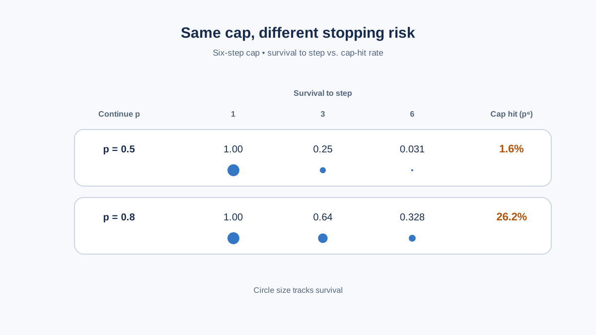
At p = 0.5 and N = 6, that's 0.5⁶ = 1.6%. The cap is nearly irrelevant — almost every run finishes on its own.
At p = 0.8 and N = 6, that's 0.8⁶ = 26.2%. More than one in four runs runs out of budget. That's not a safety net. That's a routine outcome.
Here's the trap. Both configurations have the same cap and the same per-step cost. But they have wildly different completion rates, and expected cost alone doesn't tell you which one you're in. A $0.074 average looks harmless until you realize a quarter of your users are getting truncated answers.
Common mistake: Treating "stopped" as a single outcome. There are two ways a loop stops — stopped because done and stopped because out of budget — and only the first is success. If you log only total cost, you can't tell them apart.
This is why expected cost is not a sufficient budget metric on its own. You need the cap-hit rate next to it. The pair tells a story the average can't.
Knowledge check
Check your understanding
Answer this question before you continue.
Choosing A Cap From A Cost Ceiling
Now invert the model. Suppose you have a maximum acceptable average spend per run, and you want the largest cap that keeps expected cost under it.
Start from the expected-cost formula and solve for N:
That looks intimidating, but the tradeoff it encodes is simple. Raising N buys you completion probability — more runs get to finish — and pays for it in expected spend, because the cap-hit branch is where the money goes. The typical run is cheap. The tail is expensive. Every extra step of cap is a bet that the tail is worth insuring against.
A compact decision rule when p is uncertain: estimate p as a range, then pick N for the pessimistic end. If you think p is somewhere between 0.6 and 0.8, size the cap as if it's 0.8. Uncertainty in p argues for a lower cap, not a higher one, because the cost curve is convex in p — the bad case is worse than the good case is good.
Warning: An expected-cost ceiling is not a hard per-run spend limit. With fixed per-step cost c and cap N, the model's worst-case spend is cN. If you need a hard ceiling on any single run, you must satisfy cN ≤ your limit — or enforce the budget with a pre-call gate that blocks the next step before it fires. The formula above limits the average; it does not cap the maximum.
Knowledge check
Check your understanding
Answer this question before you continue.
Where The Toy Model Breaks
Everything above is a consequence of three assumptions. Here's what happens when you drop them.
p is not constant. Real loops get more likely to continue when they're confused and more likely to stop when they're close to done. That means the geometric model understates the long tail (confused runs drag on) and overstates the short tail (easy runs finish faster than p suggests). The single-number p is a summary that hides the shape.
Per-step cost is not uniform. Context grows as the loop runs, so later steps carry more tokens than earlier ones. The true cost curve bends upward. A model that assumes flat c will underestimate the cost of long runs — precisely the runs you were worried about.
Steps are not independent. A failed step changes the state the next step sees. This is the assumption that matters most for design, because it's the reason structured feedback can help and raw retries often don't. If step 3 fails and step 4 sees the same state, you've paid for a reroll. If step 4 sees a diagnosis of why step 3 failed, you've paid for information.
The cap may not be enforced where you think. A pre-call gate that blocks the next step before it fires produces a different worst-case overshoot than a post-hoc trace that notices the cap was exceeded after the fact. The model assumes the cap is a hard wall. In practice, it's often a suggestion.
Warning: The model tells you what to measure, not what your system will do. It licenses claims like "if continuation probability is roughly constant at 0.8, a cap of 6 implies about a quarter of runs truncate." It does not license claims about your production loop without measuring p from your own traces.
Turning The Model Into A Budget You Can Defend
The math is only useful if it changes what you do on Monday.
Estimate p from traces, not from intuition. Count the steps in your last few hundred runs and fit the survival curve. If the empirical curve looks geometric, the model applies. If it has a fat tail, you've found a real signal — some subset of tasks is genuinely harder, and a single p is the wrong abstraction.
Track cap-hit rate as a first-class metric. Average cost tells you what you spend. Cap-hit rate tells you whether the cap is doing real work or just sitting there. If it's near zero, your cap is loose and you're paying for insurance you don't need. If it's high, you're truncating real work and the cap is a product decision, not just a cost control.
Enforce the cap outside the loop. A budget the agent can skip is not a budget. Put the gate where the agent can't route around it.
Know when to stop looping entirely. If p is high and the task is well-defined, iteration is buying variance, not quality. A fixed workflow with a clear sequence of steps will finish more reliably and cost less. The loop earns its place only when the task genuinely requires the agent to decide what to do next based on what it just learned.
The honest next step is to instrument a loop you already have. Log the step count for every run. Plot the survival curve. Compare it against the geometric prediction. If they match, you can budget with the formula above. If they don't, you've learned something more valuable than a number: you've learned where your model of your own system is wrong.
Knowledge check
Final check
Finish the article by checking the ideas you just learned.
References
Want a more structured LLMOps path?
Use the LLMOps Practical Starter Bundle to connect RAG, evaluation, observability, and production patterns.
Large Language Models Starter Pack
A 12-chapter guide connecting LLM fundamentals with prompting, RAG, agents, tool calling, evaluation, security, and application engineering.
- 227-page Illustrated PDF edition
- 12 guided LLM engineering chapters
- Visual concept diagrams
- Self-assessment quizzes
- Bonus deep-dive sections
- Prompt design, structured output, context windows & RAG pipelines
- Agents, tool calling, prompt injection, evaluation & application lifecycles
Coming soon


