LLM Scaling Laws: Work Through a Simple Scaling Example

You have seen the chart. A straight line on a log-log plot, a caption promising that more compute buys predictable improvement, and a comment section arguing about whether the line will hold. The chart is real. The problem is what you think it promises.

A scaling relationship is a fitted summary of many training runs. It is not a law of nature, and it is not a forecast for the next model. Once you can separate those three things, the chart becomes genuinely useful — and you stop asking it questions it was never built to answer.

Let's define the quantities, state the assumptions, and then run a calculation you can redo by hand.

What a Scaling Relationship Actually Claims

Three ideas get merged in most scaling headlines, and the merge is where the confusion starts.

A fitted trend is a curve drawn through observed results from many training runs. A training recipe is the set of choices — architecture, optimizer, data mix, schedule — that produced those runs. A capability claim is a statement about what a model can do on a task.

A scaling relationship lives in the first category. It says: across this family of runs, under these fixed choices, loss moved in this pattern as size and data grew. It does not describe a recipe, and it does not describe a capability.

If you already know what parameters are, you have the right starting point. Parameter count is one input to the fit. It is not the output, and it is not a score. The fit takes parameter count, training tokens, and training compute, and produces a predicted loss.

Those three quantities are also not independent. Training compute is roughly a function of model size and the number of tokens processed, so you cannot freely turn one dial without moving the others. That coupling is exactly why scaling questions get interesting — and why "just make it bigger" is not a strategy.

Note: A scaling relationship describes average behavior across a family of runs under fixed training choices. Change the family, and you are reading a different curve.

Notation and Assumptions Before Any Numbers

Before any arithmetic, define the symbols. Skipping this step is how people end up comparing two numbers that were never comparable.

Symbol	Meaning	Plain-language reading
N	Number of parameters	How much capacity the model has to store learned structure
D	Training tokens	How much text the model actually saw during training
C	Training compute	Roughly the total work spent on the training run
L	Loss	A number that measures how surprised the model is by the next token

A widely used simplified form looks like this:

$L = E + \frac{A}{N^{\alpha}} + \frac{B}{D^{\beta}}$

Read it term by term.

E is the irreducible floor. It is the loss you would approach with infinite parameters and infinite data on this data distribution and tokenizer. It is not zero, because natural language has genuine uncertainty in it.

A/N^α is the model-capacity term. As parameters grow, this term shrinks — but it shrinks slowly, because α is typically a small positive number. That small exponent is the whole story of diminishing returns.

B/D^β is the data term. It behaves the same way: more tokens help, but each additional token helps less.

The constants A, B, α, and β are fitted from data. They are not derived from first principles. They are what you get when you draw a line through observed runs.

Why the axes are logarithmic

Plot loss against parameters on ordinary axes and you get a curve that looks like it is flattening into nothing. Plot both on logarithmic axes and the power-law terms become straight lines. A straight line on a log-log plot is the visual signature of a power law, and it is also a visual warning: constant visual progress on that axis means multiplicative growth in the underlying quantity.

The assumptions you are accepting

Every number below depends on these holding:

• A fixed architecture family
• A fixed tokenizer
• A fixed training recipe
• A fixed data distribution
• A loss metric that is comparable across runs

Change the tokenizer and the fitted constants no longer transfer. Change the data mix and the same is true. This is not a technicality — it is the boundary of the model's authority.

Worked Example: Two Points on One Curve

The constants below are chosen for arithmetic, not lifted from any specific published fit. The shape is what matters.

Let:

• E = 1.5
• A = 200, α = 0.30
• B = 400, β = 0.30

Start with a small model: N = 1 (in units of 10⁹ parameters) and D = 100 (in units of 10⁹ tokens).

Model-capacity term:

$200 / 1^{0.30} = 200$

Data term:

$400 / 100^{0.30}$

Since $100^{0.30} = 10^{0.60} \approx 3.98$:

$400 / 3.98 \approx 100.5$

Total loss:

$L = 1.5 + 200 + 100.5 \approx 302$

Now scale parameters by 10x, keeping data fixed at D = 100. So N = 10.

Model-capacity term:

$200 / 10^{0.30} \approx 200 / 2.00 = 100$

Data term: unchanged at ≈ 100.5

Total loss:

$L = 1.5 + 100 + 100.5 \approx 202$

Ten times the parameters cut loss by about 100 points.

Now reset to N = 1 and scale data by 10x instead. So D = 1000.

Data term:

$400 / 1000^{0.30} = 400 / 10^{0.90} \approx 400 / 7.94 \approx 50.4$

Model-capacity term: unchanged at 200

Total loss:

$L = 1.5 + 200 + 50.4 \approx 252$

Ten times the data cut loss by about 50 points.

What the two deltas tell you

At this point on the curve, ten times the parameters produced roughly twice the loss reduction that ten times the data did. That is a real, checkable result — and it is also temporary.

But read that carefully. It is a statement about loss change under this formula, not a statement about which change is a better use of a fixed training budget. The two changes may require different amounts of compute, and this example does not model that constraint. A compute-matched comparison is a different question, and it needs a different calculation.

Push further. Set N = 100 and D = 1000.

Model-capacity term:

$200 / 100^{0.30} = 200 / 10^{0.60} \approx 200 / 3.98 \approx 50.3$

Data term: ≈ 50.4

Total loss:

$L = 1.5 + 50.3 + 50.4 \approx 102$

Now add another 10x of parameters, to N = 1000, with data still at 1000.

Model-capacity term:

$200 / 1000^{0.30} \approx 200 / 7.94 \approx 25.2$

Total loss:

$L = 1.5 + 25.2 + 50.4 \approx 77$

The parameter term is now smaller than the data term, and the next 10x of parameters will buy even less. The two terms have swapped roles. The bottleneck moved.

Here is the same curve as a table, so you can see the flattening without plotting anything:

N (params)	D (tokens)	Capacity term	Data term	Total loss
1	100	200.0	100.5	302.0
10	100	100.0	100.5	202.0
1	1000	200.0	50.4	252.0
100	1000	50.3	50.4	102.2
1000	1000	25.2	50.4	77.1

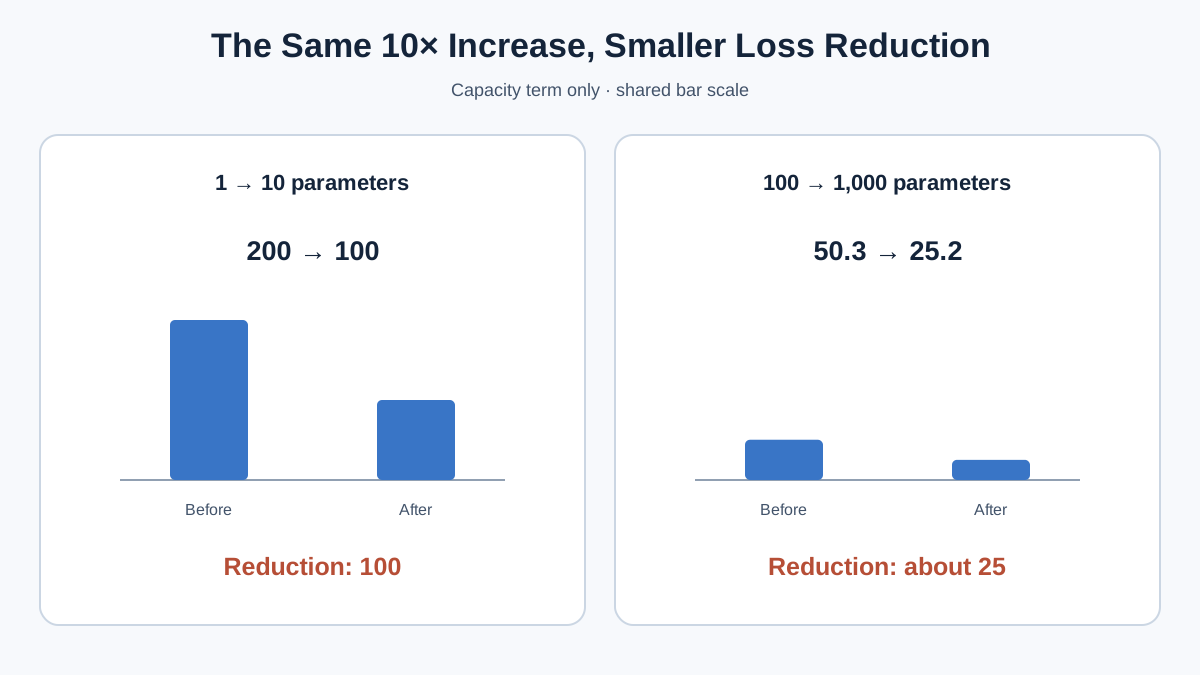
Read the last two rows together. Going from 100 to 1000 parameters — another 10x — cut loss by about 25 points. The first 10x cut it by 100. Same multiplier, a quarter of the return.

Common mistake: Treating the first 10x result as the general rule. The return on parameters depends on where you already are on the curve. There is no fixed exchange rate between parameters and loss.

Reading the Curve Correctly: What It Predicts and What It Does Not

The fit predicts a loss value under stated conditions. That is the entire claim.

It does not predict benchmark scores. It does not predict whether a model will follow instructions, write working code, or reason through a multi-step problem. Those are different quantities measured by different instruments.

The loss-to-capability gap

Loss improves smoothly. Capability does not have to.

Some tasks track the loss curve closely — text generation quality and perplexity tend to move with it. Some tasks saturate early, like simple sentiment classification, where the model hits a ceiling long before the loss curve flattens. Some tasks stay flat and then shift, because they depend on a capability that only appears once the model has enough of something else.

This is why you cannot extrapolate a task curve from a loss curve. You can predict the loss of a larger model with reasonable confidence. Predicting whether it passes a specific evaluation requires knowing how that evaluation relates to loss — and that relationship is task-specific.

The uncertainty you should carry

Fitted constants carry error bars. Extrapolating several orders of magnitude past the fitted range is an assumption, not a result. The curve is a summary of a region you have actually explored. Outside that region, you are drawing a line and hoping.

Tip: Use the curve to compare training budgets inside a known family. Do not use it to promise a feature.

Why Training Trends Do Not Set Your Deployment Cost

This is the most expensive misreading of a scaling chart.

Training compute and inference cost are different quantities driven by different variables. Training scales with the run — a one-time cost that ends when the run ends. Inference scales with usage — a cost that recurs every time someone sends a request.

Parameters affect memory footprint and per-token compute. But so do latency targets, throughput requirements, batching strategy, quantization, and hardware choice. A larger model can be cheaper per request if it needs fewer retries or produces shorter outputs. A smaller model can be more expensive if it fails often enough that you pay for three attempts to get one usable answer.

Consider a hypothetical comparison. Model A is larger and gets the task right on the first attempt with a short output. Model B is smaller and needs two or three attempts with longer outputs before producing something usable. Per token, Model A costs more. Per successful task, Model A may cost less.

That is the number that matters. Cost per successful task, not cost per parameter.

Common mistake: Reading a training-compute chart and concluding something about API pricing or self-hosting cost. The chart describes the training run. Your bill describes your usage.

Common Misreadings and How to Catch Them

Keep this list close the next time a scaling headline crosses your screen.

Treating a fitted trend as a physical law. The curve is a summary of observed runs. It has no obligation to continue.

Comparing across different tokenizers, data mixes, or evaluation setups. If the constants were fitted under different conditions, the comparison is not meaningful.

Assuming a fixed loss improvement means a fixed capability improvement. The mapping from loss to task performance is not uniform across tasks.

Extrapolating far past the fitted range and reporting the result as a prediction. Beyond the explored region, you are assuming, not measuring.

Confusing compute-optimal allocation with capability-optimal allocation. A training run can be efficient by one measure and poorly suited to your product goal by another. The allocation that minimizes loss for a fixed compute budget is not automatically the allocation that gives you the capability you need.

When to Use This Model and When to Reach for Something Else

Use a scaling relationship when you are comparing training budgets inside one model family, sanity-checking a compute claim someone made, or explaining why returns diminish as you scale.

Do not use it to choose a model for a product, estimate serving cost, or predict whether a specific task will succeed. For those questions, the right tools are different: evaluation on your own task, measured latency and cost under realistic load, and task-specific testing.

The curve is a map of a region, not a route to a destination. It tells you what the terrain looked like where you have already walked. It does not tell you what is over the next ridge.

So the next time you see a scaling claim, ask four questions. Which quantity was fitted? Over what range? Under which assumptions? And is the question you actually care about loss, task performance, or deployment cost?

If the answer is anything other than loss, close the chart and go test the model on your own task. That is the only measurement that speaks to the question you are actually asking.