
Temperature and Token Sampling: The Probability Math
Temperature does not add randomness to a model. It reshapes a probability distribution the model already produced — and once you see the arithmetic, you…

Key topics
Temperature does not add randomness to a model. It reshapes a probability distribution the model already produced — and once you see the arithmetic, you stop treating the dial as a creativity knob.
You already know the intuition: low temperature means predictable output, high temperature means varied output. That sentence is true and almost useless. It does not tell you why a logit gap of 2 becomes a probability ratio of 54.6 at one setting and 2.7 at another, or why lowering temperature can make a wrong answer more consistent rather than more correct.
To reason about that, we need the actual mechanism. The good news: it is one equation, and a four-token example carries the whole story.
From Logits to Probabilities: The Baseline Softmax
Before temperature enters, the model produces a vector of logits — raw, unnormalized scores, one per token in the vocabulary. Call them , where is the vocabulary size. Logits are not probabilities. They can be negative, they do not sum to anything meaningful, and their absolute values carry no interpretation on their own.
To turn logits into a probability distribution, we apply the softmax function:
Two properties make the exponential the right choice here. First, is always positive, so every token gets a non-negative probability. Second, the exponential is strictly increasing, so if , then . Softmax preserves the ranking of the logits — it only changes their scale.
Let's pin this down with a running example. Suppose the model has narrowed the next token to four candidates, with these logits:
| Token | Logit |
|---|---|
| Paris | 5.0 |
| London | 4.0 |
| Berlin | 3.0 |
| banana | 1.0 |
At the baseline (no temperature adjustment), we compute of each logit: , , , . The denominator is their sum: .
Dividing through gives the baseline distribution: Paris ≈ 0.657, London ≈ 0.242, Berlin ≈ 0.089, banana ≈ 0.012. That is the distribution the model actually produced. Everything from here is about how temperature transforms it.
Knowledge check
Check your understanding
Answer this question before you continue.
The Temperature Formula, Term by Term
The temperature-scaled softmax is:
Read the numerator carefully. Temperature divides the logits, not the probabilities. This is the single most common point of confusion. If you think temperature multiplies the output probabilities, you will predict the wrong behavior at every setting.
Because the division happens before the exponential, temperature controls how much the logit gaps matter. To see this, take any two tokens and and form their probability ratio:
The denominator cancels. What remains is a clean statement: temperature only affects the relative gap between logits. It never changes which token ranks highest. If Paris has the largest logit at , it has the largest logit at every positive temperature. Temperature changes the spread, not the order.
A few boundary cases follow directly from that ratio:
- is the identity case. The formula reduces to the baseline softmax.
- makes the ratio explode for the top token. The distribution collapses toward the argmax — greedy selection.
- makes every ratio approach 1. The distribution flattens toward uniform.
Note: is a limit, not a value. You cannot divide by zero, so implementations handle it as a special case — usually by switching to greedy decoding or clamping to a small positive number. When you set temperature to 0 in an API, you are asking for argmax, not for the formula to be evaluated at zero.
One more thing worth flagging early: providers do not apply temperature at the same point in the pipeline. Some scale logits before truncation (top-k or top-p), some after. The same numeric temperature is not portable across APIs, and I have watched that assumption cause real debugging pain.
Knowledge check
Check your understanding
Answer this question before you continue.
Worked Example: One Distribution, Three Temperatures
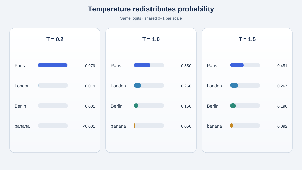
Let's run the four-token example through three temperatures. I will show in full, then tabulate the rest.
At , we divide each logit by 0.2, which is the same as multiplying by 5. The scaled logits become 25.0, 20.0, 15.0, and 5.0. Now exponentiate: , , , .
The denominator is dominated by the first term: roughly . Dividing through gives Paris ≈ 0.993, London ≈ 0.0067, Berlin ≈ 0.000045, banana ≈ 0.000000002.
Here is the full comparison:
| Token | Logit | P(T=0.2) | P(T=1.0) | P(T=1.5) |
|---|---|---|---|---|
| Paris | 5.0 | 0.993 | 0.657 | 0.553 |
| London | 4.0 | 0.0067 | 0.242 | 0.284 |
| Berlin | 3.0 | 0.000045 | 0.089 | 0.146 |
| banana | 1.0 | ~0.000000002 | 0.012 | 0.038 |
Look at what happened to banana. At it is effectively unreachable. At it has a 3.8% chance — small, but real. Same logits. Different world.
The ratio formula explains the shift. Take Paris and Berlin, a logit gap of 2. At , their probability ratio is : Paris is roughly 55 times more likely. At , the same gap gives : Paris is now less than three times more likely. Temperature did not touch the logits. It changed how much the gap mattered.
This is the formal version of what people loosely call "creativity." Lower temperature concentrates probability mass on the top tokens; higher temperature spreads it across the tail. The technical name for that concentration is entropy, and temperature is a direct lever on it — not a linear one, but a monotonic one.
Knowledge check
Check your understanding
Answer this question before you continue.
What Sampling Actually Does With Those Probabilities
Here is where a lot of confusion lives: the model outputs a distribution, and the sampler draws one token from it. These are two separate steps, and temperature only touches the first.
Greedy decoding ignores the distribution entirely. It takes the argmax. If your pipeline uses greedy, temperature is irrelevant — you can set it to anything and the output will not change.
Stochastic sampling draws from the distribution. This is where temperature matters, and it is also where variation comes from. The same prompt at the same temperature can produce different tokens on different runs. That is not model inconsistency; it is the sampler doing its job.
Truncation methods sit alongside temperature and reshape the candidate set:
- Top-k keeps only the highest-probability tokens and renormalizes.
- Top-p (nucleus sampling) keeps the smallest set of tokens whose cumulative probability exceeds .
The interaction between temperature and truncation depends on order. If temperature is applied first, it changes which tokens survive the truncation cut. If truncation is applied first, temperature only redistributes mass within the surviving set. Providers differ here, and the difference is observable.
Common mistake: Assuming a fixed seed guarantees reproducibility. On some platforms it does, but not when the model is genuinely uncertain between near-equal candidates. I have seen runs with a fixed seed and near-zero temperature still diverge on questions the model was "wrestling with." Determinism is a property of the whole pipeline, not a parameter you can set and forget.
Knowledge check
Check your understanding
Answer this question before you continue.
Sampling Variation Is Not Correctness
This is the section I would underline twice if I were handing you the article on paper.
Temperature changes which plausible token gets picked. It does not change which token is correct. Those are different questions, and conflating them is the most expensive mistake in this territory.
Consider a factual question where the model is confidently wrong. Its distribution puts high probability on the wrong answer. Lowering temperature makes that wrong answer more consistent — you get the same error every time, which feels like reliability but is just reproducibility. Raising temperature gives you a chance of sampling a different token, but only if the correct answer was already somewhere in the distribution with non-trivial mass. If it was not, no temperature setting will surface it.
The mirror failure is creative work. At low temperature, the model keeps picking the same high-probability token, and the output goes flat and repetitive. Raising temperature adds variety — and also adds incoherence risk, because you are now sampling from the tail where the model's judgment is weakest.
The decision rule I use:
Temperature controls the shape of the output distribution, not the content of the answer. If the model has the right answer somewhere in its distribution, temperature helps you sample it. If it does not, temperature is the wrong dial.
Correctness comes from the prompt, the context, the model's knowledge, and — when you need external facts — retrieval. Temperature is downstream of all of those.
When to Reach for Temperature — and When Not To
Rough guidance, with the caveat that provider defaults differ and the numbers are not portable:
| Goal | Temperature range | Why |
|---|---|---|
| Structured extraction, classification, deterministic pipelines | 0 – 0.3 | You want the highest-probability token almost every time |
| Code generation where one correct form exists | 0 – 0.3 | Same reasoning; variation is usually error |
| General chat, drafting, summarization | 0.7 – 1.0 | Some variation is acceptable and often useful |
| Brainstorming, creative writing, generating diverse candidates | 1.0 – 1.5 | You want the tail to have real probability mass |
The more important guidance is when not to reach for temperature at all. If the problem is a vague prompt, missing context, or a model that simply does not know the answer, changing temperature is a distraction. You will spend an afternoon tuning a dial that cannot fix the actual bottleneck. I have done this. It feels productive. It is not.
Also remember that temperature interacts with top-p and top-k. Tuning one in isolation can mislead you, because the other two may be doing most of the work.
What the Math Cannot Tell You
The formula describes how temperature transforms a given distribution. It says nothing about whether that distribution is well-calibrated, whether the model's logits reflect reality, or whether the top token is actually the right answer. Those are separate questions, and the math is silent on all of them.
Provider implementations vary in ways that matter. Some clamp temperature to a maximum. Some apply frequency or presence penalties before truncation, some after. Some treat as greedy, others clamp to a tiny positive value. The same number is not the same behavior across APIs, and treating it as portable is a reliable way to ship a bug.
Sampling settings are also one lever among many. Prompt quality, context, model choice, and retrieval quality usually dominate the outcome. If you are debugging a bad response, I would check those first and reach for temperature last.
One open question worth watching: reasoning-style models may not expose or honor the temperature parameter the same way standard models do. The behavior is evolving, and the safe assumption is that the parameter's effect is model-specific until you have tested it.
The One Question That Replaces the Dial
Before you touch temperature, ask a single question: is the problem distribution shape or distribution content?
If the model has the right answer somewhere in its distribution and you just need to sample it more reliably, temperature is your lever. Lower it for consistency, raise it for variety, and watch the ratio formula predict what happens.
If the model does not have the right answer in its distribution, temperature is the wrong dial. Fix the prompt, add context, retrieve better evidence, or choose a different model. The math will not save you from a distribution that never contained the answer.
The best way to internalize this is to run it. Take the four logits from this article — [5.0, 4.0, 3.0, 1.0] — and compute the softmax at three temperatures in a notebook. Change one value. Watch the probabilities shift. The formula stops being abstract the moment you have executed it and seen the numbers move.
Knowledge check
Final check
Finish the article by checking the ideas you just learned.
References
Want a more structured LLMOps path?
Use the LLMOps Practical Starter Bundle to connect RAG, evaluation, observability, and production patterns.
Large Language Models Starter Pack
A 12-chapter guide connecting LLM fundamentals with prompting, RAG, agents, tool calling, evaluation, security, and application engineering.
- 227-page Illustrated PDF edition
- 12 guided LLM engineering chapters
- Visual concept diagrams
- Self-assessment quizzes
- Bonus deep-dive sections
- Prompt design, structured output, context windows & RAG pipelines
- Agents, tool calling, prompt injection, evaluation & application lifecycles
Coming soon


