Practice Reconstructing an LLM Application Run from a Trace

A bad answer arrives. The trace UI shows a tree. You still cannot say which step did the damage.

That gap is the whole exercise. Reading a trace and reconstructing a run are different skills. One is browsing. The other is archaeology: you take a flat pile of recorded events, order them, read the numbers, and point at the step that most likely broke — while being honest about what the evidence does and does not prove.

Here is the drill. One compact JSONL file, one Python 3.11 script using only the standard library, one concrete failure to localize. No API keys, no tracing vendor account, no external services. By the end you will have a reconstructed request path, a timing and usage summary, and one localization claim with the trace fields that support it.

State the constraint up front and hold it: this exercise produces localization evidence, not a root-cause verdict. Localization narrows the search to a step. Proof comes later, from a controlled change and a re-run.

Note: This assumes you already know what a span, a trace, and a run are. If those terms are still fuzzy, the observability background is worth a pass first. Everything below builds on that vocabulary rather than re-teaching it.

The Trace File and Its Fields

Before any code, look at the data. A compact JSONL trace is one JSON object per line, one line per event. Here is a short excerpt — one retrieval event, one tool event, and two model events, with parent references forming a chain:

{"run_id":"r-7","event_id":"e1","parent_id":null,"step":"request","start":0.000,"end":0.010,"status":"ok"}
{"run_id":"r-7","event_id":"e2","parent_id":"e1","step":"retrieval","start":0.012,"end":0.240,"status":"ok","doc_ids":["d-88","d-91"]}
{"run_id":"r-7","event_id":"e3","parent_id":"e1","step":"tool","start":0.242,"end":0.410,"status":"ok","tool":"order_lookup"}
{"run_id":"r-7","event_id":"e4","parent_id":"e1","step":"model","start":0.412,"end":1.980,"status":"ok","input_tokens":3120,"output_tokens":180}
{"run_id":"r-7","event_id":"e5","parent_id":"e1","step":"model","start":1.982,"end":2.640,"status":"ok","input_tokens":640,"output_tokens":95}

The fields that matter for this exercise:

Now the traps. Timestamps may be recorded in different units or from different clocks, so a duration computed across two steps can be nonsense. A parent_id may be missing, or it may point at a step that never logged. Usage fields may be absent on some step types — retrieval and tool steps often carry no token counts at all.

And the deepest trap: the trace records what each step did, not what it relied on. Execution order is usually recoverable from timestamps and parent links. The dependency layer — which passage a model actually used, what state a tool read — is rarely logged. Keep that boundary in mind, because it is exactly where overclaiming starts.

Picture the file as a flat list of lines and the run as a tree: the root request at the top, retrieval, tool, and model hanging beneath it. Your job is to turn the flat list back into that tree, in order.

Build the Inspection Script

Here is the smallest useful version. It loads the file, groups events by run, sorts them, and prints a timeline with per-step duration and both token counts.

import json
from pathlib import Path

def load_events(path):
    events, dropped = [], 0
    for line in Path(path).read_text().splitlines():
        line = line.strip()
        if not line:
            continue
        try:
            events.append(json.loads(line))
        except json.JSONDecodeError:
            dropped += 1
    return events, dropped

def fmt_tokens(value):
    return "-" if value is None else str(value)

def timeline(events, run_id):
    run = [e for e in events if e.get("run_id") == run_id]
    run.sort(key=lambda e: e.get("start", float("inf")))
    for e in run:
        start, end = e.get("start"), e.get("end")
        dur = f"{end - start:.3f}s" if start is not None and end is not None else "n/a"
        print(f"{e.get('step','?'):<10} {e.get('event_id','?'):<4} "
              f"parent={str(e.get('parent_id')):<5} {dur:>8} "
              f"status={e.get('status','?'):<6} "
              f"in={fmt_tokens(e.get('input_tokens')):>5} "
              f"out={fmt_tokens(e.get('output_tokens')):>4}")

events, dropped = load_events("trace.jsonl")
print(f"loaded={len(events)} dropped={dropped}")
timeline(events, "r-7")

Expected output for the excerpt above:

loaded=5 dropped=0
request    e1   parent=None  0.010s status=ok     in=    - out=   -
retrieval  e2   parent=e1    0.228s status=ok     in=    - out=   -
tool       e3   parent=e1    0.168s status=ok     in=    - out=   -
model      e4   parent=e1    1.568s status=ok     in= 3120 out= 180
model      e5   parent=e1    0.658s status=ok     in=  640 out=  95

Three implementation choices are doing real work here. Reading line by line means one malformed line costs you one event, not the whole file — and you count what you dropped instead of hiding it. Grouping by run_id isolates one request from whatever else shares the file. Sorting by start gives you a candidate order, not a guaranteed one.

That last point deserves emphasis. Sorting by timestamp is a hypothesis. Clock skew can reorder steps that actually ran in sequence, and equal timestamps leave sibling order ambiguous. When the parent chain and the timestamps disagree, trust the parent chain for structure and the timestamps for duration — and say so in your notes.

Reconstruct the Run and Read the Numbers

Now turn the timeline into a sentence a human can follow. For run r-7: the request came in, retrieval returned two documents, a tool looked up an order, a first model hop ran with 3,120 input tokens and produced 180 output tokens, and a second model hop produced the final answer with 640 input tokens and 95 output tokens.

That is the request path. Reading it aloud is not busywork — it forces you to notice what is missing. There is no step between the two model hops that re-checks the first hop's output. There is no step that validates the tool result. The path is short, and every gap in it is a candidate location.

Durations are signals, not decoration. Compare them:

• Total run time is roughly 2.64 seconds. The first model hop alone is 1.568 seconds — about 59 percent of the run.
• Retrieval is 0.228 seconds. Fast. Retrieval speed is not the problem here.
• The tool call is 0.168 seconds. Also fast.

If retrieval had dominated, you would look at the vector store or the query. Here, the model hop dominates, which points your attention at prompt assembly and generation.

Usage is the second signal. The first model hop's 3,120 input tokens against the second hop's 640 is a large drop. That pattern is consistent with a bloated first prompt — a full context dump — followed by a lean follow-up. It is also consistent with a retry that re-sent a large context. The trace alone cannot tell you which; it can only tell you the first hop carried a lot of input. Treat it as a lead, not a conclusion.

Flag the gaps explicitly. A step with no end timestamp never reported completion. A parent_id that never appears as an event_id means part of the tree is missing. A tool call with no matching result event means the result was never logged — or never happened.

Localize the Failure Without Overclaiming

The trace tells you the shape of the run. To localize a failure, you need one more input: the actual content behind the IDs. Here is the accompanying fixture for run r-7 — the retrieved passages and the final answer, supplied alongside the trace so every premise is inspectable.

d-88: "Duplicate charges are refunded automatically within 3 business days."
d-91: "Refunds appear on your statement within 5-7 business days."

final_answer: "There is no duplicate charge on your account."

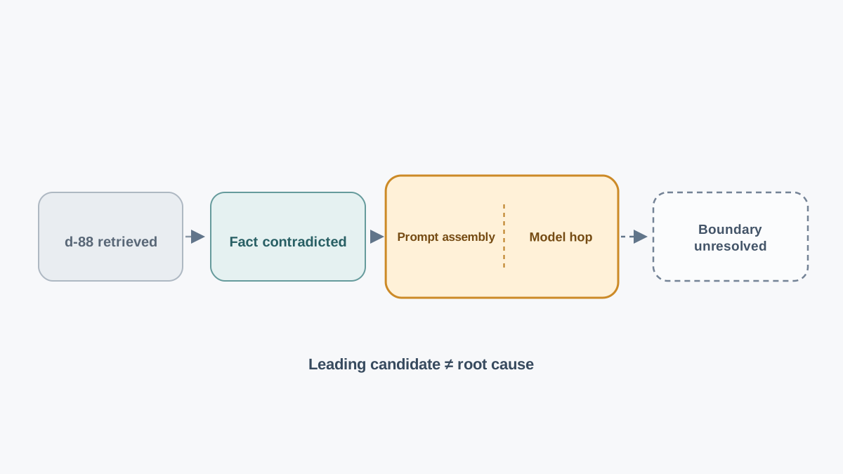
Now the concrete failure. The final answer contradicts a fact that the retrieved passage actually contained. Retrieval returned d-88 and d-91, and the correct fact — that duplicate charges are refunded automatically — was in d-88. So the evidence was present. The answer still got it wrong.

Two candidate locations:

1. Retrieval. Did it return the right passage? The doc_ids field says yes — d-88 is there. This candidate is weakened by the trace itself.
2. Prompt assembly or the model hop. The right passage was available, but the answer contradicts it. The damage most likely happened where the passage was assembled into the prompt or where the model generated over it.

Write the localization as a claim with evidence attached:

Localization claim: The failure most likely occurred at the first model hop (e4). Supporting fields: retrieval (e2) returned doc_ids: ["d-88","d-91"], and d-88 contains the contradicted fact; e4 recorded input_tokens: 3120, consistent with a large assembled context; no step in the run re-checks the model's claim against the retrieved passage.

Then write the falsifier — what would confirm or kill this hypothesis:

• If the assembled prompt for e4 shows d-88 was truncated or dropped, the location moves to prompt assembly.
• If a re-run with the same retrieval and a trimmed prompt produces a correct answer, the hypothesis survives.
• If the same contradiction appears even when d-88 is the only passage in context, the location moves inside the model hop itself.

Common mistake: Treating the last step before the bad output as the cause because it is closest to the damage. Recency is not causality. The second model hop (e5) is the last step, but it received the first hop's output — the corruption likely predates it.

The decision rule that keeps you honest: if the trace cannot distinguish two candidate steps, the honest output is a ranked shortlist, not a single verdict. Here the trace distinguishes retrieval from generation, so a single leading candidate is defensible. It does not distinguish prompt assembly from generation, so that boundary stays open.

Failure Modes in the Exercise Itself

Do not confuse failures in the traced application with failures in your own reconstruction. They look similar and mean different things.

• Malformed or truncated JSONL lines. Skip and count them. Report how many were dropped. A silent skip is a lie about coverage.
• Missing parent ids. Fall back to timestamp ordering and mark the reconstruction as lower confidence. Do not invent a parent.
• Mixed timestamp units or timezones. Detect this by comparing individual step durations against total run duration. If a step's duration exceeds the whole run, your units are wrong.
• Duplicate or retried events with the same step type. Decide whether they are retries or parallel branches before ordering them. Two model events with the same parent may be sequential hops or a retry of one hop.
• Absent usage fields. Report usage as partial, not zero. A missing input_tokens field means the count was not recorded, not that no tokens were used.

Each of these is a reconstruction failure, not an application failure. Fix the script before you blame the system.

Extend the Drill

One modification deepens the skill more than any other: add a second run to the file and diff the two timelines. If the failure path is stable across runs, you have a reproducible case. If it is not, you are looking at non-determinism, and a single trace was never going to be enough.

Two smaller extensions worth doing:

• Add a check that flags any step whose duration exceeds a threshold you choose, and justify the threshold. A threshold you cannot defend is noise.
• Turn the script into a small reusable inspector you can point at any JSONL trace, keeping it standard-library only. The value compounds when the same tool works on every file you collect.

Note the boundary. This drill localizes failures in recorded evidence. Deciding what to change, and proving the change helped, belongs to evaluation and regression work — different tools, different questions.

What to Do Next

The habit transfers: reconstruct first, cite fields second, claim cause last. That order is what separates debugging from guessing.

Run the script on a trace from your own application. Pick one failure, write one localization claim with the fields that support it, and state the falsifier you would need to confirm or kill it. If you cannot write the falsifier, you have not localized anything yet — you have only found a suspicious step.

From here, the natural next moves are comparing runs to see whether a failure is stable, and evaluating whether a fix actually improved the behavior. Both build directly on the reconstruction skill you just practiced.