
Approximate Nearest-Neighbor Search: Recall, Memory, and Latency Tradeoffs
A retrieval system answers in four milliseconds over a million vectors. Your first instinct is that the index must be computing similarity faster than…

Key topics
A retrieval system answers in four milliseconds over a million vectors. Your first instinct is that the index must be computing similarity faster than brute force. It isn't. It is checking far less of your data — on purpose.
That distinction is the whole article. Approximate nearest neighbor search is not a smarter similarity function. It is a search-space navigation strategy that deliberately skips most of the collection and bets that the vectors it skipped were not the ones you needed. Once you see the bet clearly, the recall, memory, and latency numbers stop looking like vendor magic and start looking like a budget you chose.
We will define the exact baseline, build one bounded graph model by hand, trace a query through it, and then read the tradeoffs off that model instead of memorizing benchmark tables.
The Baseline You Are Approximating
Exact top-k search is the ground truth. Given a collection of vectors, a query , a similarity or distance function , and an integer , exact search scores against every vector in and returns the best. Call that result set .
The dominant cost is the linear scan: similarity computations, one per vector. Selecting the top from those scores is a separate, cheaper step — you can maintain a bounded heap of size in time, or sort all scores in if you want the full ranking. Either way, the scan dominates, and the cost grows linearly with regardless of any index structure. No graph, no tree, no hash — just arithmetic repeated times.
You already know where the ranking comes from: a chosen measure such as dot product, cosine similarity, or Euclidean distance turns geometry into an ordered list. That part is settled. The question is what happens when grows into the millions, dimensionality grows into the hundreds or thousands, and your per-query latency budget stays in the milliseconds.
Exact search does not become wrong at that scale. It becomes expensive. And that is the framing that matters: exact search is not the slow option — it is the definition of correct. Approximation only means something relative to it. If you cannot compute the exact answer, you cannot say how much accuracy you gave up.
Knowledge check
Check your understanding
Answer this question before you continue.
Recall@k: The Only Honest Scorecard
Recall@k measures how much of the exact answer your approximate index actually found:
where is the approximate result set and is the exact top-k. The numerator counts how many true neighbors survived; the denominator is how many you were supposed to return.
A micro-example makes it concrete. Exact top-5 returns . Your ANN index returns . Recall@5 is . You found three of the five vectors that exact search would have found, and you spent two result slots on vectors that were not in the true top five.
Two things about this number get misused constantly.
First, recall is a per-query quantity. A single query's recall is noisy — 0.6 on one query tells you almost nothing. You average recall over a query set, and the query set has to resemble production traffic. Tuning until recall@10 looks high on twenty hand-picked queries, then discovering those queries were unrepresentative, is the most common way teams fool themselves.
Second, recall@k is a retrieval-fidelity metric, not a relevance metric. It measures whether the index found the vectors exact search would have found. It says nothing about whether those vectors contain the answer to the user's question. A perfect recall@k against bad embeddings or bad chunking still hands the model useless evidence.
Common mistake: Treating recall@k as an accuracy score for the whole retrieval system. It scores one layer — the index — against one reference point — exact search on the same vectors.
Knowledge check
Check your understanding
Answer this question before you continue.
A Bounded Graph Model of ANN Search
Most production ANN indexes are navigable proximity graphs, and the model is small enough to hold in your head.
Each stored vector is a node. Each node keeps links to a selected set of neighbors. The index is the graph — the links — not a second copy of your data. Two parameters carry most of the behavior:
- Graph degree: how many neighbor links each node keeps.
- Search breadth: how many candidate nodes the query keeps alive while exploring.
The query procedure is a greedy walk. Enter at a start node. Score its neighbors against . Move to the closest neighbor found. Repeat from there. Stop when no neighbor improves on the current best, then return the best nodes seen along the way.
That is the entire speedup. The walk touches a small, parameter-controlled number of nodes instead of all . The bound is the mechanism.
This model rests on assumptions worth stating plainly, because they are also the failure modes:
- The graph is navigable — from a reasonable entry point, each hop can get you closer to the query.
- The similarity measure is meaningful for your data.
- The query distribution resembles the data distribution used to build the graph.
Break the first assumption and the walk gets trapped in a poorly connected region, stopping at a local minimum that is nowhere near the true neighbor. Break the third and a query far outside the indexed distribution has no good entry path — the graph has nothing to navigate toward.
Knowledge check
Check your understanding
Answer this question before you continue.
Walking a Small Graph by Hand
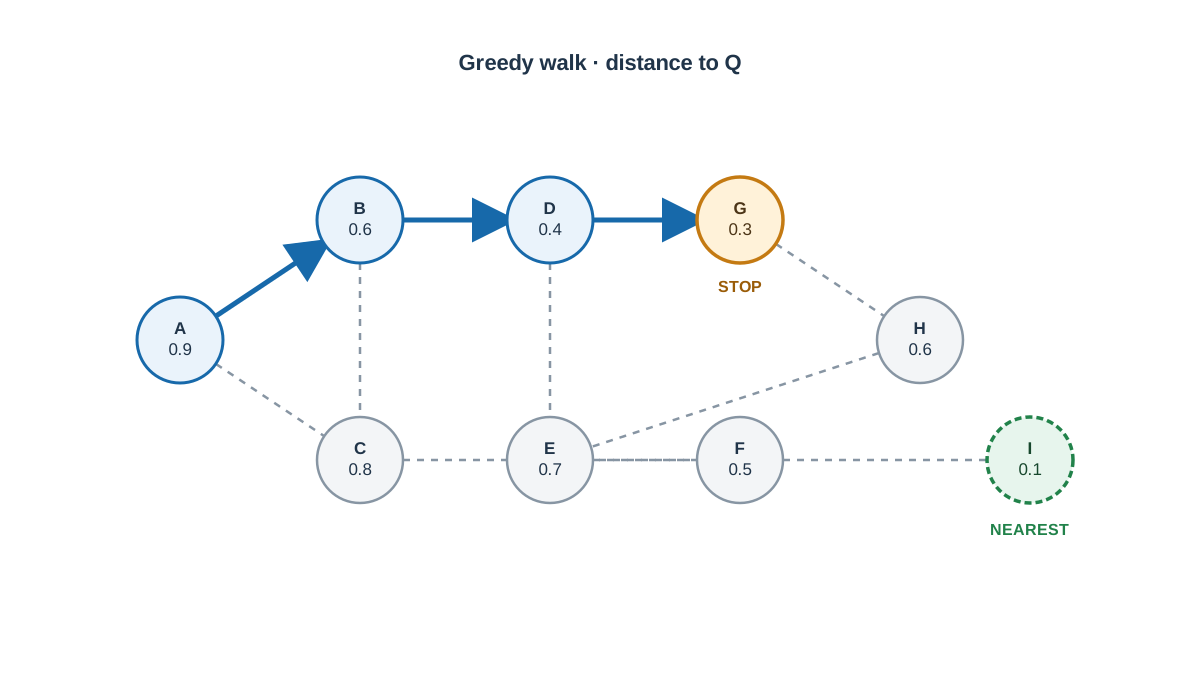
Nine nodes, one query, distances given as plain numbers. Node is the query point; the numbers are distances from to each node.
| Node | Distance to Q | Neighbors |
|---|---|---|
| A | 0.9 | B, C |
| B | 0.4 | A, D, E |
| C | 0.7 | A, F |
| D | 0.2 | B, G |
| E | 0.5 | B, H |
| F | 0.6 | C, I |
| G | 0.3 | D |
| H | 0.8 | E |
| I | 0.1 | F |
Exact top-3. Score every node: I (0.1), D (0.2), G (0.3). So .
The walk. Start at A (0.9). Neighbors B (0.4) and C (0.7). B is closer, so move to B. From B, neighbors are A (0.9), D (0.2), E (0.5). D is closer, so move to D. From D, neighbors are B (0.4) and G (0.3). G is closer, so move to G. From G, the only neighbor is D (0.2) — worse than G's 0.3. No improvement. The walk stops at G.
Best three nodes visited: G (0.3), D (0.2), B (0.4). So .
Recall@3. , so recall@3 .
The walk missed node I, the true nearest neighbor at distance 0.1. Look at why: I is reachable only through F, and F is reachable only through C. The walk went A → B → D → G and never took the A → C branch. The math was never wrong. The search was bounded, and the bound cut off the path to the best answer.
That is the tradeoff in miniature, and it is worth drawing: nodes as circles, links as lines, the walk path highlighted, the stopping node marked, and I sitting one unvisited branch away.
Knowledge check
Check your understanding
Answer this question before you continue.
Turning the Two Dials: Degree and Search Breadth
The two parameters move different costs.
Higher graph degree means more links per node. That costs memory — the index stores more connections — and it costs build work, because constructing a good graph requires repeated neighbor searches during insertion. What you buy is a better-connected graph that the walk can navigate more reliably.
Higher search breadth means the query keeps more candidates alive and explores more of the graph. That raises recall and raises per-query latency. It does not change index memory at all.
| Parameter | Recall | Query latency | Index memory | Build time |
|---|---|---|---|---|
| Higher degree | ↑ | ~flat | ↑ | ↑ |
| Higher breadth | ↑ | ↑ | flat | flat |
The dials interact, which is where most tuning goes wrong. Raising degree without raising breadth may barely help — you built better roads but the query still refuses to drive far. Raising breadth on a sparse graph wastes latency wandering dead ends. And build time is a third axis entirely: it grows with degree and with collection size, and it is the cost you pay once but feel during every reindex.
The practical reading: recall is bought with latency at query time, or with memory and build time at index time. No configuration improves all four at once.
Reading a Cost Table Without Fooling Yourself
Here is an illustrative table — not a benchmark of any specific library or dataset. Real numbers depend on dimensionality, dataset, hardware, and query distribution.
| Configuration | Recall@10 | p50 latency | Index memory |
|---|---|---|---|
| Low degree, low breadth | 0.82 | 1 ms | 1.0× |
| Medium degree, medium breadth | 0.94 | 3 ms | 1.4× |
| High degree, high breadth | 0.99 | 9 ms | 2.1× |
Read it in this order: pick the row that meets your latency budget first, then check whether its recall is acceptable for your task. Not the reverse. The highest-recall row is usually the wrong default, because the last few points of recall often cost disproportionate latency and memory for a retrieval step whose output gets re-ranked or read by a model anyway.
Below roughly a hundred thousand vectors, exact search is often fast enough that the operational complexity of tuning an ANN index is not worth it. Above that, the tradeoff becomes real and you have to choose a point on the curve deliberately.
Warning: Recall numbers from two systems built on different embeddings or different ground-truth query sets are not comparable. If the ground truth differs, you are measuring two different things and calling them the same name.
Retrieval Fidelity Is Not Relevance
A high-recall index can still produce a bad RAG answer, and knowing which layer to debug is the difference between a fix and a week of wasted tuning.
The layers are independent: embedding quality, chunking, index recall, and generation each fail on their own. Recall@k measures whether the index found the vectors exact search would have found — not whether those vectors contain the answer. A perfect index cannot rescue chunks that split a table from its header or embeddings that never learned your domain's vocabulary.
Debug in this order. First, verify that exact search returns useful evidence for your queries. If it doesn't, the index is not your problem. Second, measure how much recall the ANN index loses against that exact baseline. Third, and only then, tune degree and breadth.
Treat recall as a budget you spend, not a score you maximize. Decide the minimum acceptable recall for your task, then buy the cheapest configuration that clears it.
What to Do Next
Run exact search on a sample of your own queries to produce ground truth. Measure recall@k for one approximate configuration. Then change exactly one parameter — search breadth — and re-measure recall and latency. Watch the shape of the curve, not a single point.
Before you tune anything else, write down the minimum recall your application can tolerate. That number is your budget, and everything after it is arithmetic.
When you are ready to look above the index, the next thing to inspect is the layer that feeds it: how your documents are chunked and how your embeddings are produced. Those decisions set the ceiling that no amount of index tuning can raise.
Knowledge check
Final check
Finish the article by checking the ideas you just learned.
References
Want a more structured LLMOps path?
Use the LLMOps Practical Starter Bundle to connect RAG, evaluation, observability, and production patterns.
Large Language Models Starter Pack
A 12-chapter guide connecting LLM fundamentals with prompting, RAG, agents, tool calling, evaluation, security, and application engineering.
- 227-page Illustrated PDF edition
- 12 guided LLM engineering chapters
- Visual concept diagrams
- Self-assessment quizzes
- Bonus deep-dive sections
- Prompt design, structured output, context windows & RAG pipelines
- Agents, tool calling, prompt injection, evaluation & application lifecycles
Coming soon


