Embedding Similarity Math: Dot Products, Cosine, and Retrieval Ranking

A retrieval system returns a top result with a similarity score of 0.83. Most people read that number as "83% relevant" or "83% likely to be correct." It is neither. It is a geometric measurement between two lists of numbers, and once you can compute it by hand, you stop trusting the number and start trusting the ranking.

This article assumes you already know that embeddings turn meaning into vectors. Here we work on the arithmetic of comparing them: how the score is built, how a similarity measure turns a pile of candidate vectors into an ordered list, and why a high score is evidence of similarity, not proof of truth.

What the Similarity Score Actually Measures

An embedding places a piece of text as a point in a high-dimensional space. Comparing two embeddings means comparing two arrows: how aligned are they, and how far apart do their tips sit?

A similarity score answers one narrow question: how aligned are these two vectors? It does not answer "is this document true," "is this the answer," or "should the model trust this." Those are separate judgments that happen after retrieval, not inside the score.

To keep every calculation visible, we will use a tiny 3-dimensional vector set as a stand-in for real embeddings, which often have hundreds or thousands of dimensions. The arithmetic is identical; only the number of terms changes.

Three measures show up constantly in retrieval work, and they are related but not interchangeable:

• Dot product — the sum of component-wise products.
• Cosine similarity — the dot product with vector length divided out.
• Euclidean distance — the straight-line distance between vector tips.

We will derive the first two and use the third as a reference point.

Notation and Assumptions Before We Calculate

A vector is an ordered list of numbers. We write a vector $a$ with components $a_1, a_2, \dots, a_n$, where $n$ is the dimension — the number of numbers in the list.

The dot product of two vectors multiplies matching components and sums the results:

$a \cdot b = a_1 b_1 + a_2 b_2 + \dots + a_n b_n$

The magnitude (length) of a vector is the square root of the vector dotted with itself:

$\|a\| = \sqrt{a \cdot a} = \sqrt{a_1^2 + a_2^2 + \dots + a_n^2}$

Three assumptions matter for everything that follows:

1. Vectors are real-valued and non-zero.
2. The query and the documents were embedded by the same model.
3. Both sides share the same dimension $n$.

Warning: Comparing vectors from different models, or vectors with different dimensions, is meaningless. The numbers do not share a coordinate system, so any score you compute is noise dressed as arithmetic.

Deriving the Dot Product Step by Step

Let's compute a dot product on real numbers. Suppose our query vector is:

$q = [1, 2, 3]$

And one candidate document vector is:

$d = [2, 1, 4]$

Multiply matching components and add:

$q \cdot d = (1)(2) + (2)(1) + (3)(4) = 2 + 2 + 12 = 16$

That is the whole calculation. A large positive dot product means the vectors point broadly in the same direction and/or are long. Both effects are baked into the same number.

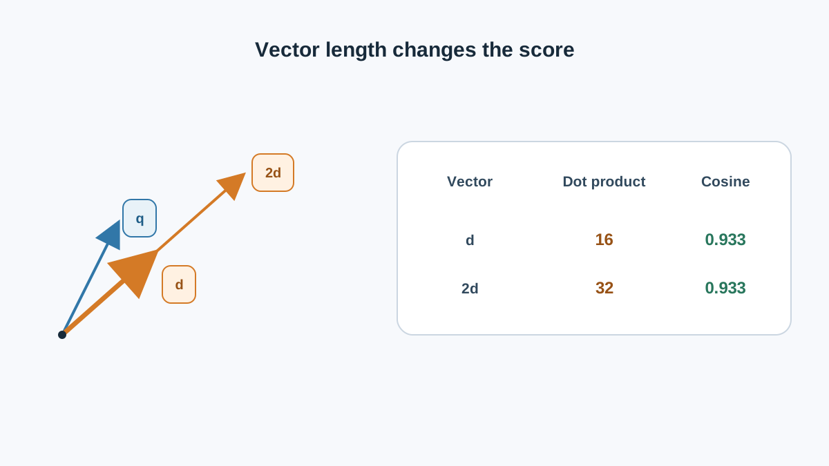
Here is the trap. Take a document vector that is simply longer, but pointed in the same direction:

$d' = [4, 2, 8]$

$q \cdot d' = (1)(4) + (2)(2) + (3)(8) = 4 + 4 + 24 = 32$

The dot product jumped from 16 to 32, but $d'$ is just $d$ scaled by 2. The score doubled because the vector got longer, not because it got more relevant. This is why raw dot product is sensitive to magnitude, and why some systems use it deliberately: when length carries a real signal — popularity, frequency, recency — you may want that signal in the score. When length is noise, you do not.

Deriving Cosine Similarity from the Dot Product

The dot product has a geometric identity behind it:

$a \cdot b = \|a\| \, \|b\| \cos\theta$

where $\theta$ is the angle between the two vectors. Rearranging isolates the cosine:

$\cos\theta = \frac{a \cdot b}{\|a\| \, \|b\|}$

That expression is cosine similarity. It is the dot product with both lengths divided out, so only direction survives.

Let's compute it for $q = [1, 2, 3]$ and $d = [2, 1, 4]$. We already have $q \cdot d = 16$. Now the magnitudes:

$\|q\| = \sqrt{1^2 + 2^2 + 3^2} = \sqrt{14} \approx 3.742$

$\|d\| = \sqrt{2^2 + 1^2 + 4^2} = \sqrt{21} \approx 4.583$

Divide:

$\cos\theta = \frac{16}{3.742 \times 4.583} \approx \frac{16}{17.15} \approx 0.933$

The result is bounded. Cosine similarity runs from -1 (opposite directions) through 0 (orthogonal, no shared direction) to 1 (identical direction). Because length is divided out, a long document and a short document can score identically if they point the same way — which is usually what you want for text embeddings, where document length is not a signal of relevance.

Worked Example: Ranking Three Documents Against One Query

Now let's turn the formula into a nearest neighbor retrieval ranking. Keep the query:

$q = [1, 2, 3]$

And add three candidate documents:

$d_1 = [2, 1, 4], \quad d_2 = [3, 3, 3], \quad d_3 = [-1, 0, 1]$

Cosine similarity for $d_1$ we already computed: $\approx 0.933$.

Cosine similarity for $d_2$:

$q \cdot d_2 = (1)(3) + (2)(3) + (3)(3) = 3 + 6 + 9 = 18$

$\|d_2\| = \sqrt{9 + 9 + 9} = \sqrt{27} \approx 5.196$

$\cos\theta = \frac{18}{3.742 \times 5.196} \approx \frac{18}{19.44} \approx 0.926$

Cosine similarity for $d_3$:

$q \cdot d_3 = (1)(-1) + (2)(0) + (3)(1) = -1 + 0 + 3 = 2$

$\|d_3\| = \sqrt{1 + 0 + 1} = \sqrt{2} \approx 1.414$

$\cos\theta = \frac{2}{3.742 \times 1.414} \approx \frac{2}{5.29} \approx 0.378$

Sort descending: $d_1$ (0.933), $d_2$ (0.926), $d_3$ (0.378). The retrieval rule is plain: the highest score wins the top slot. Take the top $k$ and hand them to the next stage.

Now re-run the same comparison with raw dot product:

Document	Dot product	Cosine similarity
$d_1$	16	0.933
$d_2$	18	0.926
$d_3$	2	0.378

The ranking flips at the top. Dot product puts $d_2$ first because it is longer; cosine puts $d_1$ first because it points more directly at the query. Neither is "wrong." The measure you choose is a design decision about what you want the score to reward.

Why High Scores Are Not Proof of Relevance

Here is the misconception that causes the most damage: treating the score as an absolute measure of relevance or truth.

Many embedding models compress scores into a narrow high band. In practice, unrelated sentence pairs from some models can still land above 0.7, because the model was trained to push relevant pairs higher than irrelevant ones — not to spread scores across the full -1 to 1 range. A 0.75 can be a weak match in one model and a strong one in another. The absolute number is not portable across models.

Note: What matters is the relative order of scores, not their absolute values. An embedding model is useful as long as relevant pairs score higher than irrelevant pairs, even when the gap is small.

That gives you a practical rule: use scores to form a model-specific candidate ordering, then evaluate whether that ordering serves your task. Thresholds must be calibrated per model and per dataset, usually by inspecting the score distribution on your own data rather than borrowing a cutoff from a blog post.

The score also cannot answer three separate questions:

• Is this relevant? The score is evidence, not a verdict.
• Is this correct? Similarity is not truth. A confidently wrong passage can sit close to the query.
• Is this sufficient to answer the user? Retrieval finds candidates; it does not decide whether they cover the question.

Choosing a Measure and Knowing When It Breaks

The decision rule is short:

• Use cosine similarity when direction should dominate and length is noise — the usual case for text embeddings.
• Use dot product when length carries real signal, such as popularity or frequency, and you want that signal in the score.

One simplification is worth memorizing: if you normalize every vector to unit length, the dot product and cosine similarity produce the same ranking. Many vector indexes exploit this by storing normalized vectors and using a fast inner-product search.

Failure modes to watch:

• Mixing embedding models. Query and documents must come from the same model.
• Comparing across dimensions. Different $n$ means no shared space.
• Unnormalized vectors in a dot-product index. Length silently dominates the ranking.
• Treating a score as a probability. It is not one, and it does not sum to anything meaningful across candidates.

Common mistake: Setting a hard similarity threshold and assuming everything above it is relevant. Calibrate the threshold on your own data, or skip the threshold and rely on top-$k$ ranking plus a re-ranking step.

That last point is the practical bridge. Retrieval is a coarse filter. The usual way to recover precision is to retrieve more candidates than you need, then re-rank them with a stronger, slower model. The math in this article gets you a good shortlist; it does not get you a final answer.

What to Do Next

Compute the score. Rank the candidates. Then judge the ranking, not the number.

Here is a concrete exercise that will teach you more than another article. Start with the toy vectors from this article: $q = [1, 2, 3]$, $d_1 = [2, 1, 4]$, $d_2 = [3, 3, 3]$, $d_3 = [-1, 0, 1]$. Compute both dot product and cosine similarity for each pair by hand. Confirm the ranking flip you saw in the table. Then change one component of $d_3$ and watch how the ranking shifts.

Once the arithmetic feels mechanical, embed three short sentences with a single model — one that clearly matches a query, one loosely related, one unrelated — and compare the model's cosine scores to your hand calculations. If the unrelated sentence scores surprisingly high, you have just seen the narrow-band problem in your own data, and you will never read a similarity score the same way again.

From here, the next design problem is ranking quality: how many candidates to retrieve, how to re-rank them, and how to measure whether the top slot is actually the one you want.