
RAG Retrieval Metrics: Precision, Recall, Reciprocal Rank, and NDCG
Two retrievers return the same relevant chunk. One puts it at rank 1; the other buries it at rank 4. A single "accuracy" number calls them identical. The…

Key topics
Two retrievers return the same relevant chunk. One puts it at rank 1; the other buries it at rank 4. A single "accuracy" number calls them identical. The metric you pick decides which failure you can see.
You already know how to eyeball retrieved chunks and ask whether they look relevant. That skill gets you through a demo. It collapses the moment you have fifty queries, two embedding models, and a reranker to justify. Now we put numbers on the ranking — and, just as important, we choose numbers that expose the failure we actually care about.
Why One Retrieval Score Lies to You
Fix the setup before touching a formula. You have one query, a corpus of chunks, and a retriever that returns the top results in order: . You also have a set of chunks that are genuinely relevant to the query — the ground truth.
That last piece is not optional. Every metric in this article is computed by comparing the retrieved list against . Without relevance labels, these metrics do not exist. You can still judge retrieval by hand or with a model as a judge, but you cannot compute precision, recall, reciprocal rank, or NDCG. Building the labeled set is usually the real work; the arithmetic is the easy part.
A ranked list hides two independent failure modes:
- Coverage — relevant evidence never made it into the list at all.
- Ordering — relevant evidence is present but buried under noise.
Any single number collapses both into one value. That is why "our retrieval accuracy is 0.8" tells you almost nothing. The rest of this article derives four metrics, each answering a different question about the same list, and each blind to a different failure.
Precision@k: How Much of the Context Window Is Signal
Precision@k asks: of the items I retrieved, how many are relevant?
The numerator counts relevant items in the top ; the denominator is itself.
Work an example. Let , and suppose the retriever returns three relevant chunks and two irrelevant ones. Then:
Each retrieved slot contributes if it is relevant and if it is not. Three relevant slots give .
Interpretation: precision measures what the generator is forced to read. The model has a limited context window, and every irrelevant chunk spends tokens that could have carried evidence. Low precision means the generator is reading noise.
Precision alone is gameable. A retriever that returns exactly one perfect chunk and stops scores precision while ignoring every other relevant source. That is a coverage failure wearing a perfect score.
Common mistake: reporting precision without stating . Precision@3 and precision@10 are different measurements. A bare "precision = 0.8" is not a number you can act on.
Knowledge check
Check your understanding
Answer this question before you continue.
Recall@k: Did the Evidence Even Make It Into the List
Recall@k asks the opposite question: of all the relevant chunks that exist, how many did I retrieve in the top ?
The numerator is identical to precision's. Only the denominator changes — from to the size of the full relevant set.
Run it on the same query. Suppose the corpus contains eight relevant chunks total, so , and the retriever found three of them in the top 5:
Same numerator, different denominator, visibly different meaning. Precision asked "how clean is the list?" and answered . Recall asks "how complete is it?" and answers . The retriever is finding a little more than a third of the evidence that exists — and no amount of reranking will fix that, because the missing chunks were never in the list to reorder.
The tradeoff is mechanical. Raise and you usually pull in more relevant chunks — recall climbs — while diluting the list with irrelevant ones, so precision falls. In practice is bounded by the context window and by cost: you cannot retrieve everything and hand it to the model.
Labeling granularity matters more than most people expect. If you label at the document level, recall can look healthy while the actual answer span was never retrieved. A document counts as "found" if any chunk from it appears, even when the specific passage that answers the question is missing. Chunk-level or span-level labels tell a different, harsher story. Decide your granularity before you trust the number.
Common mistake: treating high recall as proof the answer is usable. Recall says the evidence is present in the list. It says nothing about whether the generator can reach it.
Knowledge check
Check your understanding
Answer this question before you continue.
Reciprocal Rank: Rewarding the First Useful Hit
Reciprocal rank asks a narrower question: how high is the first relevant item?
If the first relevant chunk sits at rank 1, RR is . At rank 2, it is . At rank 5, it is . If nothing relevant appears in the top , RR is .
A single query's RR is thin evidence, so we average across queries to get mean reciprocal rank:
Here is a mean reciprocal rank example across three queries. The first relevant hit lands at rank 1, rank 2, and rank 5 respectively:
What MRR reveals: whether the top of the list is trustworthy. That failure mode dominates when you pass only one or two chunks to the model — if the first chunk is wrong, the answer is wrong.
What MRR misses: everything after the first relevant hit. A query with five relevant chunks where only one is found scores the same as a query with one relevant chunk found. MRR is blind to coverage by construction.
Use MRR when the generator consumes very few chunks. Do not use it to judge whether you retrieved enough evidence.
Knowledge check
Check your understanding
Answer this question before you continue.
NDCG: Grading Relevance and Penalizing Bad Order
Binary relevance — relevant or not — throws away information. A chunk that fully answers the question and a chunk that merely mentions the topic are not equal, and a metric that treats them the same cannot tell you which ordering is better.
NDCG fixes this in four steps. Build it in order.
Step 1 — Assign graded relevance. Give each retrieved item a grade. A common scheme is for a direct answer, for strong supporting evidence, for a passing mention, for irrelevant.
Step 2 — Compute gain. Gain is the relevance grade itself. Higher grade, more gain.
Step 3 — Apply a position discount. A relevant item at rank 1 is worth more than the same item at rank 4. The standard discount is . Sum the discounted gains to get DCG:
Step 4 — Normalize. Compute the DCG of the ideal ordering and divide:
Here is the definition that trips people up, so name it explicitly: IDCG@k is computed over the same retrieved items, re-sorted by grade, best first. It is the best ordering of the list you actually have. That choice matters. It means NDCG@k measures ordering quality only — it cannot reward you for a relevant chunk that never made the top , because that chunk is not in the pool being sorted. If you want NDCG to penalize missing evidence, you have to compute IDCG over the full judged relevance set at the cutoff, not just the retrieved items. Pick one convention, state it, and keep every comparison inside it.
Normalization is what makes NDCG comparable across queries with different numbers of relevant items. It lands between and .
Now a full NDCG retrieval example. Take four retrieved chunks with grades $3, 2, 0, 1k = 4$.
Compute DCG@4 term by term:
- Rank 1:
- Rank 2:
- Rank 3:
- Rank 4:
The ideal ordering sorts those same four grades best-first: $3, 2, 1, 0$.
- Rank 1:
- Rank 2:
- Rank 3:
- Rank 4:
Read that number carefully. NDCG near means your ordering is close to the best possible ordering of the items you retrieved. The gap between your DCG and the ideal DCG is your ranking headroom — how much a better reranker could recover. It is not a statement about whether you retrieved enough evidence; that question belongs to recall.
Two assumptions to respect. NDCG depends on your grading scheme, so a score computed under one labeling rubric is not comparable to a score computed under another. And it assumes the ideal ranking is well-defined, which requires that you actually labeled the relevant items.
Knowledge check
Check your understanding
Answer this question before you continue.
Reading the Four Numbers Together
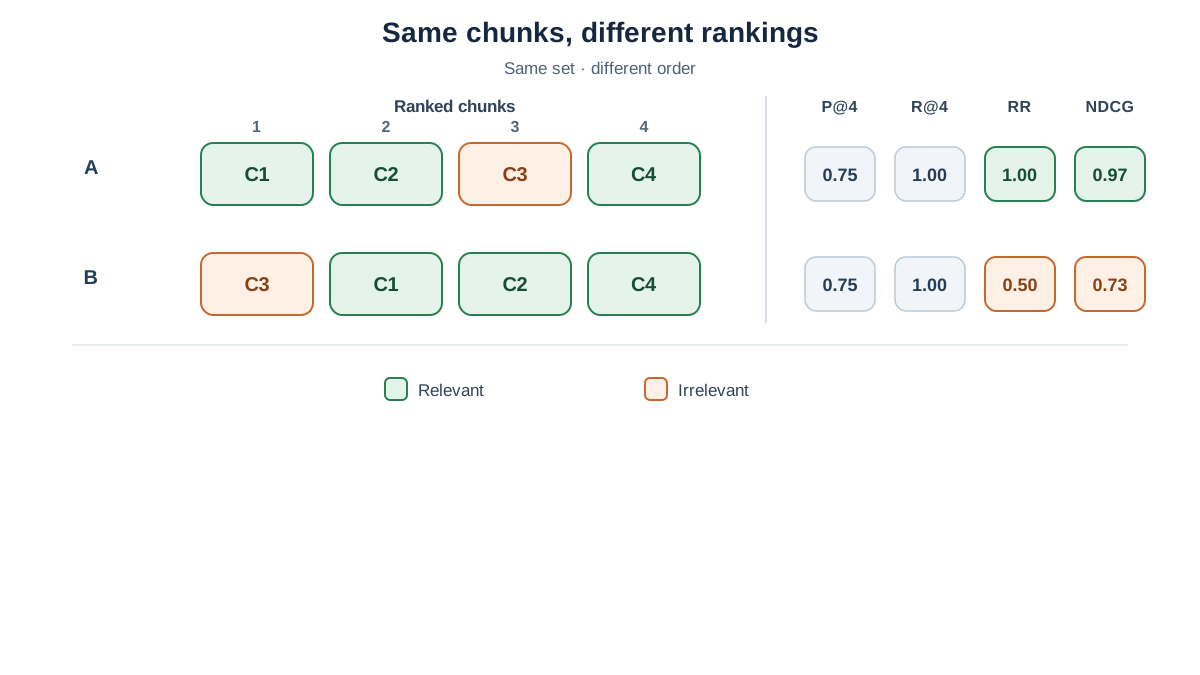
Four formulas are not four facts. They are one debugging instrument with four probes.
| Metric | Question it answers | Failure it catches | Failure it hides | Reach for it when |
|---|---|---|---|---|
| Precision@k | How clean is the top ? | Noise crowding the context | Missing evidence | You suspect the generator is distracted |
| Recall@k | Did the evidence make the list? | Missing relevant chunks | Bad ordering | Answers are wrong because evidence is absent |
| MRR | How high is the first hit? | A relevant chunk buried below noise | Everything after rank 1 | You pass one or two chunks to the model |
| NDCG@k | How close is the ordering to ideal? | Sub-optimal ranking of graded items | Missing items (under the retrieved-items convention) | You are tuning a reranker |
Now use them as a diagnostic sequence:
- Low recall → the evidence is missing. Fix chunking, embeddings, or raise .
- High recall, low precision → too much noise in the list. Add a reranker or tighten .
- High precision, low MRR or NDCG → the right chunks are present but badly ordered. Fix the reranker.
Here is the contrast that makes the point. Two retrievers return identical sets of chunks, so their precision and recall are identical. But retriever A puts the highest-graded chunk at rank 1 while retriever B puts it at rank 3. Their NDCG differs, and that difference tells you exactly what to change: B needs a better reranker, not a better embedding model.
Common mistake: optimizing a metric that does not match the failure you observe in generated answers. If answers are wrong because the evidence never arrived, a reranker will not save you. Measure the failure first, then pick the metric that exposes it.
One boundary to hold: these metrics score retrieval only. They say nothing about whether the generator used the context well. Perfect retrieval can still produce a wrong answer.
Where These Metrics Stop Being Enough
Every metric here requires relevance labels, and the quality of those labels caps the value of every score. A sloppy labeled set produces confident, precise, wrong numbers.
Aggregate scores also hide per-query disasters. An MRR of can conceal one query where retrieval failed completely. Always inspect the worst queries, not just the mean.
And retrieval metrics are blind to generation. A model that ignores or misreads the context will produce bad answers from perfect retrieval. When you see that pattern, the fix is in the prompt or the model, not the retriever.
So here is the decision rule I would give you: pick one metric that matches the failure you can actually observe, label a small query set — twenty to fifty queries is enough to start — and measure before you change chunking, , or the reranker. Change one thing. Measure again. Let the number tell you whether the change helped or just moved the problem.
The formulas are cheap. The labeled set is the asset. Build it once, and every retrieval experiment after that gets faster and more honest.
Knowledge check
Final check
Finish the article by checking the ideas you just learned.
References
Want a more structured LLMOps path?
Use the LLMOps Practical Starter Bundle to connect RAG, evaluation, observability, and production patterns.
Large Language Models Starter Pack
A 12-chapter guide connecting LLM fundamentals with prompting, RAG, agents, tool calling, evaluation, security, and application engineering.
- 227-page Illustrated PDF edition
- 12 guided LLM engineering chapters
- Visual concept diagrams
- Self-assessment quizzes
- Bonus deep-dive sections
- Prompt design, structured output, context windows & RAG pipelines
- Agents, tool calling, prompt injection, evaluation & application lifecycles
Coming soon


