Test Metadata Filters in a Small Vector Search

A filter can be correct and still delete your best evidence. Here is how to watch it happen in twenty lines of NumPy.

Most retrieval bugs I have debugged did not come from a broken embedding model. They came from a filter that did exactly what it was told. The filter matched the metadata. The scores stayed high. The ranking looked healthy. And the one chunk that actually answered the question was gone before the similarity search ever saw it.

You cannot see that failure in a vendor dashboard. You can see it in a fixture.

This is a controlled experiment. Same vectors, same query, one variable changed: the metadata filter. By the end you will have a runnable script that shows you precision, coverage, and exclusion side by side, and a decision rule for when a filter belongs in your RAG pipeline at all.

If you already know what embeddings are and how cosine similarity ranks items, you have everything you need. If not, the short version: a vector database stores numeric representations and compares them by distance, and metadata filters are the structured constraints layered on top of that comparison. We are going to isolate the filter behavior and ignore the index internals.

Why a Filter Can Improve and Destroy Retrieval at the Same Time

A metadata filter is not a soft preference. It is a hard gate. Anything outside the gate is not down-ranked; it is invisible. No similarity score, however high, can bring it back.

That single property creates the tension this whole article is about. Tighten the filter and precision often climbs, because you have removed candidates that were never going to be relevant. Tighten it further and coverage collapses, because you have also removed candidates that were relevant. At the extreme, a filter returns only relevant items because it returns almost nothing. That is not a better retrieval system. That is a system that has quietly stopped answering questions.

The dangerous case is not a wrong filter. It is a correct filter applied to a query whose best evidence lives outside the filter scope. The filter is doing its job. The retrieval is failing anyway.

Common mistake: Treating a filter as a harmless narrowing step. Narrowing is the whole mechanism, and narrowing is exactly what removes evidence.

So we need to measure two things at once: what the filter kept, and what it threw away. Precision tells you about the kept set. Coverage tells you about the thrown-away set. Report only one and you are not making a decision; you are making a guess with a number attached.

The Fixture: Vectors, Queries, Labels, and Metadata

The fixture is deliberately small. Twelve items, four dimensions, one query. You can read every score by eye, which is the point. A real index hides the mechanism behind recall curves and latency graphs. A fixture hides nothing.

Environment assumptions: Python 3.11, NumPy, no vector database, no API keys, no network calls. Everything below runs in a single file.

Here is the setup. Item vectors are hand-built so the scores are readable. The query has a known intended answer. Relevance labels mark which items actually answer the query. Metadata carries one categorical field and one numeric field, chosen so that some relevant items fall inside a plausible filter and some fall outside.

import numpy as np

# 12 items, 4 dimensions. Hand-built so scores are readable.
items = np.array([
    [0.90, 0.10, 0.05, 0.02],  # i0
    [0.85, 0.15, 0.10, 0.05],  # i1
    [0.80, 0.20, 0.15, 0.10],  # i2
    [0.20, 0.90, 0.10, 0.05],  # i3
    [0.15, 0.85, 0.20, 0.10],  # i4
    [0.10, 0.80, 0.25, 0.15],  # i5
    [0.05, 0.10, 0.90, 0.20],  # i6
    [0.10, 0.15, 0.85, 0.25],  # i7
    [0.02, 0.05, 0.10, 0.90],  # i8
    [0.05, 0.10, 0.15, 0.85],  # i9
    [0.88, 0.12, 0.08, 0.04],  # i10
    [0.12, 0.88, 0.18, 0.08],  # i11
])

query = np.array([0.95, 0.10, 0.05, 0.02])

# Ground truth: which items actually answer this query.
relevant = {0, 1, 2, 10}

# Metadata: a category tag and a year.
categories = np.array(["alpha", "alpha", "alpha", "beta", "beta",
                       "beta", "gamma", "gamma", "gamma", "gamma",
                       "beta", "beta"])
years = np.array([2021, 2022, 2023, 2021, 2022, 2023,
                  2021, 2022, 2023, 2024, 2021, 2022])

Notice the trap already baked in. Items 0, 1, 2, and 10 are relevant. Three of them are tagged alpha. One of them, item 10, is tagged beta. A filter on category == "alpha" will look reasonable and will silently drop a relevant item.

That is not a contrived edge case. That is the normal shape of real metadata.

Baseline Ranking: Cosine Similarity Without Filters

Normalize the vectors, then a single matrix operation gives you every cosine similarity at once. Normalization is what makes the dot product equal the cosine: once each vector has unit length, the dot product is the cosine of the angle between them.

def normalize(matrix):
    norms = np.linalg.norm(matrix, axis=1, keepdims=True)
    return matrix / norms

items_n = normalize(items)
query_n = query / np.linalg.norm(query)

scores = items_n @ query_n
ranking = np.argsort(-scores)

k = 5
top_k = ranking[:k]

print(f"{'rank':<5}{'item':<6}{'score':<8}{'category':<10}{'year':<6}{'relevant'}")
for rank, idx in enumerate(top_k, start=1):
    print(f"{rank:<5}i{idx:<5}{scores[idx]:<8.3f}"
          f"{categories[idx]:<10}{years[idx]:<6}{idx in relevant}")

Expected output shape:

rank item  score   category  year  relevant
1    i0    0.999   alpha     2021  True
2    i10   0.998   beta      2021  True
3    i1    0.997   alpha     2022  True
4    i2    0.995   alpha     2023  True
5    i3    0.264   beta      2021  False

Four of the top five are relevant. One is not. That is your precision baseline: 4 out of 5, or 0.80.

Now compute coverage. Coverage asks a different question: of all the items that should have been found, how many made it into the result set?

def precision_at_k(ranking, relevant, k):
    top = set(ranking[:k].tolist())
    return len(top & relevant) / k

def coverage_at_k(ranking, relevant, k):
    top = set(ranking[:k].tolist())
    return len(top & relevant) / len(relevant)

print(f"precision@5 = {precision_at_k(ranking, relevant, k):.2f}")
print(f"coverage@5  = {coverage_at_k(ranking, relevant, k):.2f}")

Baseline: precision 0.80, coverage 1.00. Every relevant item is present. The baseline is not good or bad. It is the control condition. Everything that follows is measured against it.

Applying One Metadata Filter and Reading the Damage

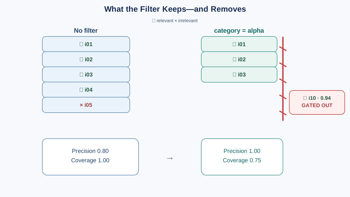
Now the experiment. Apply a single filter — category == "alpha" — as a boolean mask, restrict the candidate set, and re-rank. Same query, same vectors, one variable changed.

mask = categories == "alpha"
filtered_idx = np.where(mask)[0]
filtered_scores = scores[filtered_idx]
filtered_ranking = filtered_idx[np.argsort(-filtered_scores)]

print(f"{'rank':<5}{'item':<6}{'score':<8}{'category':<10}{'year':<6}{'relevant'}")
for rank, idx in enumerate(filtered_ranking[:k], start=1):
    print(f"{rank:<5}i{idx:<5}{scores[idx]:<8.3f}"
          f"{categories[idx]:<10}{years[idx]:<6}{idx in relevant}")

Expected output:

rank item  score   category  year  relevant
1    i0    0.999   alpha     2021  True
2    i1    0.997   alpha     2022  True
3    i2    0.995   alpha     2023  True

The filter kept only three candidates. There is no fourth or fifth row, because only three items in the entire fixture are tagged alpha. This is the first thing to notice: a filter can shrink your candidate set below k, and your ranking code has to handle that honestly instead of padding the list.

Read the numbers. Precision over the three returned items is 3 out of 3, or 1.00. Coverage is 3 out of 4, or 0.75. Item 10, which scored 0.998 in the baseline and was genuinely relevant, has vanished entirely. It was not down-ranked. It was excluded before ranking.

This is the failure mode in its purest form. The filter was semantically unrelated to the query. The query was about topic similarity. The filter was about a category tag. The two have no necessary relationship, and yet the filter dominated the outcome.

Note: The mechanism is the gate, not the score. Once an item is outside the mask, no similarity value can rescue it. This is why filter scope matters more than filter correctness.

Sweeping Filter Scope: Where Precision and Coverage Cross

One filter is a data point. A sweep is a curve. Let us vary the filter from permissive to strict and record both metrics at each step.

Here is the convention I use, and it matters: precision is measured over the returned set, not over a fixed k. When a filter returns fewer than k items, the denominator is the number of items actually returned. Padding the denominator with k would punish a filter for being selective, which is the opposite of what we want to observe. Coverage keeps its natural denominator: the number of relevant items in the whole fixture.

def evaluate(mask, label):
    idx = np.where(mask)[0]
    if len(idx) == 0:
        return label, 0.0, 0.0, len(relevant)
    ranked = idx[np.argsort(-scores[idx])]
    returned = ranked[:k]
    p = len(set(returned.tolist()) & relevant) / len(returned)
    c = len(set(returned.tolist()) & relevant) / len(relevant)
    excluded = len(relevant - set(returned.tolist()))
    return label, p, c, excluded

filters = [
    (np.ones(len(items), dtype=bool), "no filter"),
    (years >= 2021, "year >= 2021"),
    (categories == "alpha", "category == alpha"),
    ((categories == "alpha") & (years >= 2022), "alpha AND year >= 2022"),
    ((categories == "alpha") & (years >= 2023), "alpha AND year >= 2023"),
]

print(f"{'filter':<28}{'precision':<11}{'coverage':<10}{'excluded'}")
for mask, label in filters:
    label, p, c, ex = evaluate(mask, label)
    print(f"{label:<28}{p:<11.2f}{c:<10.2f}{ex}")

Expected pattern:

filter                      precision  coverage  excluded
no filter                   0.80       1.00      0
year >= 2021                0.80       1.00      0
category == alpha           1.00       0.75      1
alpha AND year >= 2022      1.00       0.50      2
alpha AND year >= 2023      1.00       0.25      3

Look at the last row. Precision is a perfect 1.00. Coverage is 0.25. Three of the four relevant items are gone. If you reported only precision, you would conclude the filter was excellent. It is the worst filter in the table.

This is the trap the sweep exposes. Precision rises as scope tightens because you are removing candidates, and some of those candidates were irrelevant. Coverage falls because you are also removing relevant ones. At some point coverage collapses toward zero while precision looks flawless.

Warning: A filter that returns only relevant items because it returns almost nothing is not a better retrieval system. It is a system that has stopped retrieving.

For RAG, the consequence is downstream. A highly selective filter starves the context window of evidence. The model receives a thin, confident-looking set of chunks and generates a fluent answer from incomplete material. The retrieval failure becomes a generation failure, and you will be debugging the wrong stage.

Common Mistakes When Testing Filters

The sweep is only useful if the experiment is clean. These are the errors that make filter tests lie to you.

Changing the query and the filter at the same time. If you tweak both, you cannot attribute the result to either. Hold the query fixed. Change one thing.

Judging filters by the top result only. The top result is often relevant even when the filter is destroying coverage. Measure precision and coverage across the labeled set, not the first row.

Assuming a filter that matches the user's words is the right filter. Metadata semantics and query semantics are different things. A user asking about "recent policy changes" may not map cleanly onto a year field, and a category tag may not align with the topic the query is actually about.

Forgetting that a correct filter can still be harmful. The filter does not need to be wrong to break retrieval. It only needs to exclude evidence the query needs.

Treating one query as evidence. One query shows you a mechanism. It does not establish a general rule. Run the sweep on several queries before you trust a filter policy.

When to Filter, When to Widen, and What to Measure Next

The experiment gives you a decision rule.

Filter when the constraint is genuinely part of the request. A date range, a tenant boundary, a document type, a permission scope — these are real constraints the user stated or the system requires. They belong in the filter.

Widen or drop the filter when the labeled relevant set is mostly outside the filter scope. That is a signal about the filter, not about your embeddings. Do not retrain the model to fix a metadata problem.

Measure precision and coverage together. A filter decision that reports only one of them is not a decision. The sweep above shows exactly why: the best-looking precision number came from the worst filter.

My rule for retrieval work is simple. If I cannot state what the filter excludes and why that exclusion is safe, I do not ship the filter. The fixture is how I find out.

Your next experiment: add a second metadata field and sweep both dimensions at once. Then compare pre-filtering against post-filtering on the same fixture. Pre-filtering restricts the candidate set before ranking; post-filtering ranks everything and discards afterward. The coverage numbers will diverge in ways that matter for how you assemble context before generation. Run it, print the table, and read the excluded column before you read the precision column.