
RAG Chunking Math: Calculate Chunk Counts, Overlap, and Token Use
A 1,500-token document with 512-token chunks and 15% overlap quietly becomes four chunks, and the same paragraph now lives in two of them. Nobody chose…

Key topics
A 1,500-token document with 512-token chunks and 15% overlap quietly becomes four chunks, and the same paragraph now lives in two of them. Nobody chose that. The arithmetic chose it.
Most beginners tune chunk size by feel. They try 512, then 256, then 1,024, and judge the results by whether answers "feel better." That is backwards. Before you argue about retrieval quality, compute the three numbers chunk size and overlap already decided for you: how many chunks exist, how many tokens you duplicated, and how much retrieval budget you just spent.
This article assumes you have already decided to use fixed-size chunking. If you are still choosing between fixed-size, recursive, and semantic strategies, that decision comes first. Here, the strategy is fixed and the question is what the numbers do.
The Three Numbers Chunk Size Already Decided
Fixed-size chunking is a sliding window over a token stream. You take the first window, step forward, take the next window, and repeat until the document ends. Everything below follows from five variables:
| Symbol | Meaning |
|---|---|
| D | Document length in tokens |
| C | Chunk size in tokens |
| O | Overlap in tokens |
| S | Step size, where S = C − O |
| N | Chunk count |
Two assumptions matter. First, we measure in tokens, not characters or words, because that is what the embedding model and the context window actually consume. Second, we assume the splitter does not snap to sentence or paragraph boundaries. Real splitters often do, so treat the formula as an upper-bound model, not a guarantee.
From these variables you get three outputs: the chunk count N, the duplicated overlap tokens, and the retrieval token budget. Compute them in code, not by asking a model to reason about them. This is deterministic arithmetic, and deterministic arithmetic belongs in a function.
Deriving the Chunk Count Formula
Start with the first chunk. It consumes C tokens and always exists as long as D > 0. That gives us one chunk before any stepping happens.
Each subsequent chunk advances by the step S = C − O. After the first chunk, the remaining content is D − C tokens. The number of additional chunks is however many steps of size S fit into that remainder:
Add the first chunk back:
The ceiling appears because the final partial window still becomes a chunk. If 100 tokens remain and the step is 436, you do not get a fraction of a chunk. You get one more chunk holding 100 tokens.
Two degenerate cases are worth naming. If D ≤ C, the document fits in a single chunk and N = 1. If O ≥ C, then S ≤ 0 and the loop never terminates — each step moves backward or nowhere. Overlap must be strictly less than chunk size. A splitter that accepts O = C without complaint is a splitter that will hang or silently truncate.
Read the formula as a tradeoff, not a score. N grows roughly linearly with D. It shrinks as overlap increases, because overlap buys boundary safety by paying in extra chunks.
Knowledge check
Check your understanding
Answer this question before you continue.
Worked Example: A 1,500-Token Document
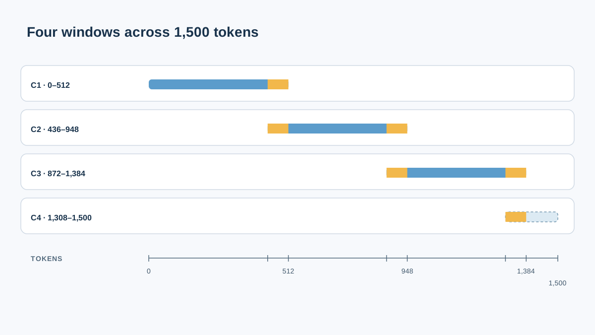
Take D = 1,500, C = 512, and O = 76 — roughly 15% overlap. Then S = 512 − 76 = 436.
Four chunks. Here is where each window starts and ends:
| Chunk | Start token | End token | Length |
|---|---|---|---|
| 1 | 0 | 512 | 512 |
| 2 | 436 | 948 | 512 |
| 3 | 872 | 1,384 | 512 |
| 4 | 1,308 | 1,500 (partial) | 192 |
Now vary one parameter at a time. Drop overlap to zero: S = 512, and N = 1 + ⌈988 / 512⌉ = 3 chunks. Raise overlap to 150: S = 362, and N = 1 + ⌈988 / 362⌉ = 4 chunks. Halve the chunk size to 256 with O = 38: S = 218, and N = 1 + ⌈1244 / 218⌉ = 7 chunks.
Notice what happened. Cutting chunk size in half more than doubled the chunk count. Raising overlap from 76 to 150 bought nothing in chunk count for this document — the ceiling absorbed it. That is the kind of thing you only see when you run the numbers.
The boundary effect is the reason overlap exists. A sentence straddling token 512 gets cut in half by chunk 1 and chunk 2. Overlap means the sentence also appears whole inside chunk 2's window. That is the mechanism, and it is worth remembering that overlap softens boundaries — it does not eliminate them.
Knowledge check
Check your understanding
Answer this question before you continue.
Counting Duplicated Tokens and the Overlap Tax
Here is where the arithmetic gets subtle, and where a lot of tutorials quietly lie to you. The nominal capacity of your index is N × C. But the actual stored tokens are the sum of the real chunk lengths — and the last chunk is often partial. For our example:
- Nominal capacity: 4 × 512 = 2,048 tokens
- Actual stored tokens: 512 + 512 + 512 + 192 = 1,728 tokens
- Duplicated tokens: 1,728 − 1,500 = 228 tokens
That is about 15% overhead, not the 37% you would get from the naive N × C estimate. The difference matters because it is the difference between a cost model you can trust and one that overstates your bill by more than double.
The general formula for actual duplication is the sum of overlaps between consecutive chunks. When every chunk is full, that sum is (N − 1) × O. When the last chunk is partial, the final overlap is truncated to whatever the partial chunk actually repeats:
For our example, the first three overlaps are each 76 tokens (228 total), and the fourth chunk is too short to contribute a full overlap. So duplication lands at 228.
Where does that overhead land? Each duplicated span gets embedded again. Overlap does not just inflate prompt size — it increases embedding calls, vector count, and storage. You pay at index time and again at retrieval time.
Common mistake: Reporting N × C as your stored-token total. That number is the ceiling your index could hold, not what it holds. If your last chunk is partial, N × C overstates both storage and duplication. Compute the actual sum of chunk lengths.
The tradeoff is plain. Overlap protects boundary evidence. The price is paid in duplicate vectors and a larger index. For most documents, 10–15% overlap is enough to soften boundaries without turning your index into a mirror.
Knowledge check
Check your understanding
Answer this question before you continue.
Turning Chunk Count Into a Retrieval Token Budget
Chunk arithmetic only matters if the retrieved chunks fit in the context window. The budget inequality:
Worked check: k = 5, C = 512 gives 2,560 retrieval tokens. Against an 8,192-token window with a 500-token system prompt and a 100-token question, 7,592 tokens remain. It fits, with room for the answer.
Now the failure case. Raise C to 1,024 and k to 8. That demands 8,192 retrieval tokens — the entire window, before the system prompt or the question. It overflows.
Overlap does not change the per-chunk retrieval cost. It changes how many chunks exist and how likely a boundary-spanning passage is retrieved twice. That second effect is subtle: two near-identical chunks can both rank highly for the same query, and you spend two slots on one piece of evidence.
Note: Stuffing more retrieved context into the prompt does not keep improving answers. Beyond a certain point, generation quality can degrade as irrelevant context dilutes the signal. Treat the budget as a constraint to respect, not a target to maximize.
My decision rule: compute the budget before raising k, and prefer raising k over raising C when precision matters. More small chunks give the retriever finer granularity. Fewer large chunks give it more context per slot but fuzzier matches.
Knowledge check
Check your understanding
Answer this question before you continue.
What the Math Cannot Tell You
The formula predicts how many chunks exist and what they cost. It says nothing about whether the right chunk ranks highly for a given query.
This is the boundary that trips people up. Chunk size effects on retrieval quality can be small or even negligible when the retrieval goal is document-level rather than passage-level. If any chunk from the correct document counts as a success, larger chunks still contain the relevant content, just with more surrounding context. The metric you choose changes the conclusion.
Boundary effects are semantic, not arithmetic. A chunk can be exactly 512 tokens and still cut a definition away from the term it defines. The math says the chunk is well-sized. The reader says the answer is wrong.
And embedding similarity is not factual correctness. A well-sized chunk can be retrieved for the wrong reason — vector closeness that looks right but misses the point.
State it plainly: the count and budget math is deterministic. The relevance consequence is empirical and must be measured on your own documents. Do the math to bound cost and catch overflow, then evaluate retrieval separately.
A Repeatable Procedure for Your Own Documents
Turn the derivation into a checklist you can run before tuning anything:
- Measure D in tokens with the same tokenizer the embedding model uses, not by word count.
- Pick C and O, compute S = C − O, then compute N. Reject any configuration where O ≥ C.
- Sum the actual chunk lengths to get stored tokens, then subtract D to get real duplication. Do not use N × C as your stored-token total.
- Check k × C against the available context window before running retrieval.
- Only after those numbers pass, evaluate retrieval quality and adjust one parameter at a time.
Three mistakes to avoid: mixing character counts with token counts, treating overlap as free, and tuning chunk size against a metric that does not match your retrieval goal.
You now own two separate jobs. The arithmetic is deterministic and belongs in code — write a function that takes D, C, and O and returns N, actual stored tokens, real duplication, and the budget check. The retrieval evaluation is empirical and cannot be inferred from chunk counts. Compute the numbers for one real document today, then measure retrieval quality as the next step. The math tells you what you can afford. Only measurement tells you whether it worked.
Knowledge check
Final check
Finish the article by checking the ideas you just learned.
References
Want a more structured LLMOps path?
Use the LLMOps Practical Starter Bundle to connect RAG, evaluation, observability, and production patterns.
Large Language Models Starter Pack
A 12-chapter guide connecting LLM fundamentals with prompting, RAG, agents, tool calling, evaluation, security, and application engineering.
- 227-page Illustrated PDF edition
- 12 guided LLM engineering chapters
- Visual concept diagrams
- Self-assessment quizzes
- Bonus deep-dive sections
- Prompt design, structured output, context windows & RAG pipelines
- Agents, tool calling, prompt injection, evaluation & application lifecycles
Coming soon


