
Model Data-Disclosure Exposure When Using an LLM
A team wants to prove that minimization is safer. So they multiply two numbers they invented, get a smaller product for the minimized option, and present…

Key topics
A team wants to prove that minimization is safer. So they multiply two numbers they invented, get a smaller product for the minimized option, and present the result as if it were a measurement of their provider. The arithmetic is fine. The claim is not. An exposure model does not tell you how likely your provider is to leak data. It tells you which of your submission options carries lower assumed loss — and only under the assumptions you wrote down.
If you have already worked through classifying sensitive data and deciding what to redact, you have done the hard part. You have a minimized version of the record. The open question is whether that reduction is worth anything, and how you would know. That is a modeling question, not a compliance question, and it has a specific shape: define your options, define your scenarios, assign assumed probabilities and impacts, and compare.
What an Exposure Model Can and Cannot Tell You
Start with the boundary, because everything downstream depends on it.
An LLM data exposure risk model answers a comparison question: given my assumptions, which submission option has lower expected loss? It does not answer: how likely is this provider to leak my data? The second question requires evidence about provider controls, retention behavior, access policies, and attacker behavior. Your arithmetic cannot produce that evidence. It can only organize what you already believe.
Three things sit outside the model entirely:
- Actual provider controls. Whether prompts are retained, for how long, under what access rules, and how they are protected.
- Actual attacker behavior. Who targets what, with what capability, and how often.
- Correlation between events. A single root cause — a misconfigured logging pipeline, for example — can trigger several scenarios at once. A sum treats them as separate contributions.
A single expected-loss number invites false confidence because it looks like a measurement. It has the format of a measurement: a number, a unit, a decimal point. But it is a product of two judgments. The durable output is not the number. It is the comparison across options, plus the assumption list that produced it.
Note: If you cannot state your assumptions in plain sentences, you do not have a model. You have a number with a story attached.
Knowledge check
Check your understanding
Answer this question before you continue.
Notation: Data Options, Scenarios, Probabilities, Impacts
Define every symbol before using it, and tie each one to something concrete in the workflow.
Data option is a candidate submission. In practice you usually have two or three: the full record, a minimized record with identifiers removed and task-relevant fields kept, and an approved substitute such as synthetic or pre-cleared data.
Scenario is a named disclosure event. Name them specifically, because vague scenarios produce vague probabilities:
- A submitted prompt is retained in logs and later surfaced to someone who should not see it.
- Model output reproduces sensitive content to a different user.
- Stored interaction data is exposed in a breach.
is the assumed probability that scenario occurs given option . The parenthetical matters: minimization changes this probability. That change is the entire point of the exercise. If your minimized option has the same as the full option, you have assumed minimization does nothing.
is the assumed impact of scenario under option , expressed in a single unit — currency, hours of remediation, or a normalized severity score. Pick one unit and keep it. If one scenario is measured in dollars and another in "reputational damage," the sum is meaningless.
Common mistake: Treating as a frequency you measured. Unless you have incident data from this exact workflow, is a judgment. Write it as one.
Knowledge check
Check your understanding
Answer this question before you continue.
Deriving Expected Exposure Loss
Build the formula from one scenario, not from a formula wall.
For a single scenario, expected loss is probability times impact:
If a scenario has a 2% assumed chance of occurring and an assumed impact of $50,000, the expected loss contribution is 0.02 \times 50{,}000 = \1{,}000. That does not mean you expect to lose \1,000. It means that if you faced this exact situation many times, the average loss per attempt would approach $1,000.
Extend to multiple scenarios by summing:
This sum is valid because expected value is linear: the expected total of a set of losses equals the sum of each loss's expected contribution. That holds whether or not the scenarios are independent, and whether or not they can co-occur — as long as each scenario's impact counts a distinct harm and you do not count the same loss twice.
That last clause is where most models break. Two failure modes matter:
Overlapping consequences. If a breach also surfaces retained prompts, and you list "breach" and "retained prompt surfaced" as separate scenarios with separate impacts, you may be counting the same dollar of harm twice. The fix is not to drop the sum. The fix is to define scenarios so their impacts partition the harm, or to fold the overlapping consequence into a single scenario.
Shared causes. A single misconfiguration can make several scenarios more likely at the same time. That does not invalidate the sum — linearity still holds. It means your individual estimates may be wrong, because you set them as if each scenario were considered in isolation. If a root cause raises three probabilities at once, the joint probability of at least one event is higher than any single suggests, and your total may understate the risk. Dependence is a problem for estimating the inputs, not for adding them.
Sensitivity weighting. Sometimes a scenario deserves more weight than its raw impact implies — a regulated identifier, for example, may trigger notification obligations that a plain dollar figure misses. If you apply a weight , write it into the formula and disclose it:
The weight is a judgment call. Hiding it inside is the same as not stating it.
Knowledge check
Check your understanding
Answer this question before you continue.
A Worked Example: Full, Minimized, and Substitute Data
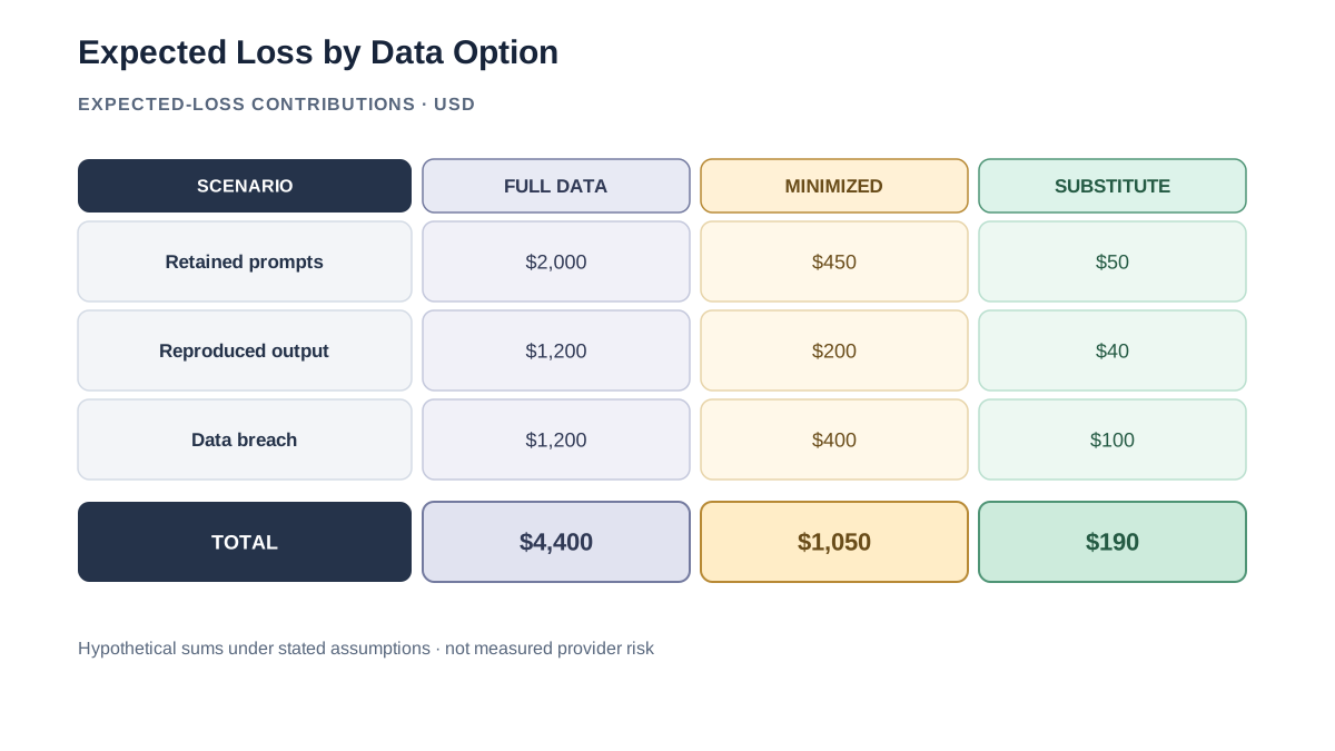
Three options, three scenarios, one unit (dollars). All numbers below are assumed, not measured. Each scenario is defined so its impact covers a distinct harm, avoiding double counting.
| Scenario | (full) | (minimized) | (substitute) | (full) | (minimized) | (substitute) |
|---|---|---|---|---|---|---|
| Prompt retained in logs, later surfaced | 0.05 | 0.03 | 0.01 | 40,000 | 15,000 | 5,000 |
| Output reproduced to another user | 0.02 | 0.01 | 0.005 | 60,000 | 20,000 | 8,000 |
| Stored interaction data breached | 0.01 | 0.008 | 0.005 | 120,000 | 50,000 | 20,000 |
Compute each option.
Full record:
Minimized record:
Approved substitute:
The gap between full and minimized is roughly $3,350 in assumed expected loss. What does that gap represent? It represents the value of removing identifiers and unnecessary fields under these assumptions. It does not represent a measured reduction in provider risk. If your probability estimates are wrong by a factor of two, the gap moves with them.
Note that the substitute option beats minimization here — but only because the assumed impacts are much lower. If the substitute data cannot support the task, that advantage is fictional. A substitute that forces rework has costs the model does not capture.
Knowledge check
Check your understanding
Answer this question before you continue.
Change One Assumption and Watch the Ranking Move
The comparison is only as stable as its weakest input. Test that directly.
Raise one probability. Suppose you learn that prompt retention is more common than you assumed, and you raise from 0.05 to 0.15. The full-record total becomes:
The ranking does not flip — minimized still wins — but the gap widens from $3,350 to $7,350. The comparison is sensitive to this assumption, and it moves in the direction that strengthens the case for minimization.
Raise one impact. Now suppose the retained identifier is a regulated one, and you raise from 15,000 to 80,000. The minimized total becomes:
Still below the full record, but the margin narrows sharply. If you also raise — because a minimized record still contains the regulated identifier — the ranking can flip.
Which assumption matters most? In this example, the comparison is most sensitive to the impact of the regulated identifier under minimization. That is the assumption worth investigating before trusting the result. A ranking that flips under a plausible assumption change is not a finding. It is a prompt to gather better evidence.
Warning: The failure mode here is tuning assumptions until the preferred option wins. If you adjust and until minimization looks best, you have not modeled anything. You have reverse-engineered a conclusion.
When This Model Helps and When It Misleads
Use it when you are comparing two or three concrete submission options, when you need to force hidden assumptions into the open, or when you are deciding where to spend effort on minimization. The model's real value is the assumption list it produces. That list is a shared artifact your team can argue about.
Do not use it when you need a real risk estimate, when you cannot name the scenarios, or when your impacts are in incomparable units. A model built on unnameable scenarios produces a number that cannot be audited or improved.
The common mistakes, collected:
- Treating as a measured frequency rather than a judgment.
- Defining scenarios whose impacts overlap, so the sum double counts the same harm.
- Setting each in isolation when a shared root cause would raise several at once.
- Hiding a sensitivity weight inside the impact figure.
- Reporting a single number without the assumption set beside it.
The honest deliverable is a comparison plus a stated assumption list — not a score. If someone asks "what is our exposure?" the correct answer is "here are three options, here are our assumptions, and here is which option wins under them."
Where to Go Next
Build the model only to compare options. Publish the assumption set next to the result. Treat any ranking that flips under a plausible assumption change as a signal to gather evidence, not as a conclusion.
The practical next step is to run this comparison on your own workflow's actual submission options. Write down the full record, the minimized version, and any approved substitute. Name three scenarios whose impacts do not overlap. Assign your best-guess probabilities and impacts, mark each one as a judgment rather than a measurement, and compute. Then change the one assumption you trust least and see whether the ranking survives.
If you want to see how the minimized option is actually constructed — which fields to strip, which to keep, and how to check for residual exposure — the practice exercise on minimizing and redacting data before an LLM request walks through that construction step by step.
Knowledge check
Final check
Finish the article by checking the ideas you just learned.
Want a more structured LLMOps path?
Use the LLMOps Practical Starter Bundle to connect RAG, evaluation, observability, and production patterns.
Large Language Models Starter Pack
A 12-chapter guide connecting LLM fundamentals with prompting, RAG, agents, tool calling, evaluation, security, and application engineering.
- 227-page Illustrated PDF edition
- 12 guided LLM engineering chapters
- Visual concept diagrams
- Self-assessment quizzes
- Bonus deep-dive sections
- Prompt design, structured output, context windows & RAG pipelines
- Agents, tool calling, prompt injection, evaluation & application lifecycles
Coming soon


