LLM Confidence Calibration: When Scores Match Correctness Rates

A confidence score is a promise about a population. Most teams read it as a promise about the answer in front of them.

That gap is where production incidents live. A system prints 0.92 next to an answer, someone downstream treats it as "roughly one error in twelve," and nobody checks whether that number was ever true across a set of predictions. The score looks like a property of the answer. It is actually a claim about a bin.

This article is about the test that decides whether the number earns its meaning. The one diagnostic handle to carry through everything below: calibration is a property of a bin, not of an answer. Once that lands, the formulas stop being arbitrary and start being obvious.

What a Confidence Score Actually Claims

Before the math, name the object precisely. A confidence score is a probability statement about a group of predictions. The formal target is:

$P(\text{correct} \mid \text{confidence} = p) \approx p$

Read it in plain English: among all predictions assigned confidence $p$, roughly a fraction $p$ should be correct. If your system emits 0.9 across a thousand answers, about nine hundred of them should be right. If only six hundred are, the number is decoration.

Two axes are hiding here, and conflating them is the most common beginner mistake. Confidence versus correctness in LLMs are separate properties. A model can be accurate and badly calibrated — right most of the time, but claiming 0.99 on everything. A model can be mediocre and well calibrated — right only 60% of the time, but honest about it. Neither axis implies the other.

If you have already worked through why one good answer proves little about dependable behavior, this is the next question in the same line of reasoning. Reliability asks whether the system works across ordinary inputs. Calibration asks whether its stated certainty tracks that reality.

Three score sources show up in practice, and we will refer back to them:

• Token logprobs — the model's probability distribution over the next token.
• Verbalized percentages — the model writing "I am 85% confident."
• Sample-agreement estimates — generating several answers and measuring how often they agree.

Each one is a different measurement of a different thing. None of them is automatically a probability of correctness.

Notation and the Two Questions Calibration Answers

Define the symbols once so the rest of the article reads cleanly.

• $N$ predictions in your evaluation set.
• $p_i$ — the confidence score assigned to prediction $i$.
• $y_i$ — the binary outcome: $1$ if correct, $0$ if incorrect.
• $B_m$ — the $m$-th confidence bin, a set of predictions whose scores fall in a range (for example, $[0.8, 0.9)$).

With that notation, calibration answers one question: do stated confidences match empirical accuracy rates? That is the $P(\text{correct} \mid \text{confidence} = p) \approx p$ condition, measured bin by bin.

A second, independent question is discrimination: do confidence scores rank correct answers above incorrect ones? A model can rank well while being systematically overconfident — it separates right from wrong, but every score is inflated. It can also rank poorly while being well calibrated — the scores are honest on average but useless for sorting.

These two properties are independent, and this is where most teams get fooled. A high AUROC (a discrimination metric) does not mean your 0.9 means 90%. It means your scores sort correctly more often than chance. Calibration and discrimination are different questions with different failure modes.

One assumption makes calibration measurable at all: you need a held-out set of cases with known correctness, and a fixed definition of "correct." If correctness itself is fuzzy or graded — a summary that is "mostly good" — calibration becomes a judgment call before it becomes a number. Decide the label first. The metric is only as honest as the label underneath it.

Reliability Diagrams: Seeing Miscalibration Before Measuring It

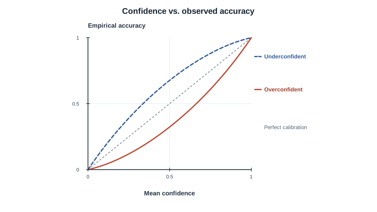
The fastest way to understand calibration is to look at it. Bin your predictions by confidence, compute the actual accuracy inside each bin, and plot the result.

Use the standard convention: mean confidence on the x-axis, empirical accuracy on the y-axis. A perfectly calibrated model produces points on the diagonal — confidence equals accuracy at every level. Real models rarely do.

With that axis convention, the direction of the error is readable:

• Points below the diagonal mean the model is overconfident: it claims more certainty than its accuracy supports. Most LLMs bow below the diagonal in high-confidence bins, and the gap is worst at the top.
• Points above the diagonal mean the model is underconfident: it is right more often than its stated confidence suggests.
• A flat curve that ignores the diagonal entirely means the score carries almost no information about correctness.

Picture three curves on one plot:

• The diagonal, for reference.
• An overconfident curve that sits below the diagonal, worst at the high end.
• An underconfident curve that rises above the diagonal in the middle and rejoins near the top.

The shape tells you which direction the error runs, and that direction tells you what to fix. Overconfidence at the top is the dangerous case, because that is where you would otherwise route to automation.

Warning: Bin count changes the picture. Too few bins hide the gap; too many bins make each bin noisy enough to mislead. Ten equally spaced bins is a common starting point, but treat the bin count as a parameter you test, not a constant you trust.

Expected Calibration Error, Derived Step by Step

The reliability diagram is visual. Expected calibration error (ECE) turns it into one number. Derive it rather than memorizing it.

Start with the per-bin gap: the absolute difference between the bin's accuracy and its mean confidence.

$\text{gap}_m = \left| \text{acc}(B_m) - \text{conf}(B_m) \right|$

A bin with 50 samples should not count as much as a bin with 5,000. Weight each gap by the share of samples in that bin:

$\text{weight}_m = \frac{|B_m|}{N}$

Sum the weighted gaps across all bins:

$\text{ECE} = \sum_{m=1}^{M} \frac{|B_m|}{N} \left| \text{acc}(B_m) - \text{conf}(B_m) \right|$

Lower is better. ECE is a weighted average absolute gap — nothing more exotic than that.

A worked example

Take 100 predictions across three bins.

Bin	Confidence	Count	Correct	Accuracy	Gap	Weight	Weighted gap
High	0.9	50	40	0.80	0.10	0.50	0.050
Mid	0.7	30	21	0.70	0.00	0.30	0.000
Low	0.5	20	12	0.60	0.10	0.20	0.020

Sum the weighted gaps: $0.050 + 0.000 + 0.020 = 0.070$.

ECE is 0.07. The mid bin is perfectly calibrated — 0.7 confidence, 70% accuracy. The high bin is overconfident by 10 points, and because it holds half the samples, it dominates the score. That is exactly where overconfidence hurts: the bin you would most want to trust is the one dragging the number up.

Notice what ECE depends on. Change the binning scheme and the number moves. Change the sample size and the noise changes. Change the correctness label and everything shifts. ECE is a summary, not a verdict.

Common mistake: Treating ECE as a single ground truth. It is sensitive to bin count and can hide compensating errors — one bin overconfident, another underconfident, canceling out in the weighted sum. The Brier score (mean squared difference between predicted probability and outcome) and maximum calibration error (the worst single bin) are complementary views. Read the curve first, then the number.

High: count 50, gap 0.10
Mid: count 30, gap 0.00
Low: count 20, gap 0.10

A Second Worked Example: Same Accuracy, Different Calibration

Here is the proof that calibration is not a restatement of accuracy. Hold accuracy fixed and change only the scores.

Two systems, same 100 cases, same 70 correct answers. System A spreads confidence across the range. System B clusters everything near 0.95.

Bin	System A conf	System A count	Correct	System B conf	System B count	Correct
High	0.9	40	30	0.95	100	70
Mid	0.7	40	28	—	—	—
Low	0.5	20	12	—	—	—

System A: gaps of $|0.75 - 0.90| = 0.15$, $|0.70 - 0.70| = 0.00$, $|0.60 - 0.50| = 0.10$, weighted $0.40 \cdot 0.15 + 0.40 \cdot 0.00 + 0.20 \cdot 0.10 = 0.08$.

System B: one bin, confidence 0.95, accuracy 0.70, gap 0.25, weight 1.0. ECE is 0.25.

Same accuracy. Three times the calibration error. System B is confidently wrong in a way System A is not, and no accuracy metric would ever show it.

The practical conclusion: a change that improves accuracy can worsen calibration, and a recalibration step can improve calibration without touching accuracy. "We got more answers right" and "our confidence numbers are trustworthy" are separate release notes. Ship them separately.

Where Confidence Scores Come From and Why They Drift

Miscalibration is not random. It has mechanisms, and once you see them you can predict it.

Token logprobs measure next-token likelihood, not the probability that a whole answer is correct. Those are different quantities. A token can be highly likely under the model's distribution while the answer it belongs to is wrong, and a low-probability token can appear in a correct answer. Treat logprobs as a model signal you can evaluate for calibration against correctness labels — not as a correctness probability by definition.

Verbalized confidence is a generated number shaped by training incentives that reward confident-sounding output. It tends to cluster near the top of the scale regardless of actual performance, and the correlation with correctness degrades further on questions where the model lacks knowledge.

Sample-agreement estimates infer confidence from consistency across multiple generations. This fails precisely when it matters most: a model that is consistently wrong will agree with itself, and agreement will read as high confidence.

Calibration is not a fixed property of a model. It shifts with task type, prompt format, domain, and model version. A model can be well calibrated on common requests and wildly overconfident on rare ones — and the rare ones are usually the ones you care about.

Tip: Segment your evaluation by query type before you trust a single ECE number. A blended score hides the segment where calibration collapses.

Calibrated Is Not Correct: Reading the Result Honestly

This is the decision boundary the article exists to establish.

Calibration is a population-level statement. It says nothing about whether this specific answer is right. A well-calibrated 0.7 still means roughly three in ten answers at that level are wrong. Calibration makes the risk legible. It does not remove it.

Three boundaries to hold:

• Calibration does not fix a weak model. A system that is right 55% of the time can be perfectly calibrated and still useless for the task.
• Calibration is measured on a distribution you chose. Shift the inputs and the guarantee weakens. The number describes your evaluation set, not the world.
• Calibration depends on your labels. If the correctness labels are wrong, the calibration number is confidently wrong too.

Where calibration earns its keep: thresholding (act only above a confidence cutoff), abstention (say "I don't know"), routing to human review, cascading to a stronger model, and showing users an honest uncertainty signal.

Where it does not: high-stakes single-shot decisions, inputs unlike your evaluation set, or any case where you have not verified the correctness labels themselves.

A Minimal Calibration Check You Can Run

Theory is only useful if it changes what you do next. Here is the smallest repeatable procedure.

1. Collect a held-out set with known correctness labels. Reuse the evaluation set you already built rather than creating a new one. If you do not have one, that is the prerequisite, not this article.
2. Record the confidence signal alongside each outcome. Keep raw signals separate — logprobs, verbalized scores, agreement rates — rather than collapsing them into one number before you know which one carries information.
3. Bin, compute per-bin accuracy, and plot the reliability curve before computing any single summary metric.
4. Read the curve first, then the ECE number. The shape tells you which direction the error runs; the number tells you how large it is.
5. Set a success criterion in advance. The curve should track the diagonal within a tolerance you chose before looking, and the ECE should be stable when you change the bin count. If it swings, your sample is too small or your bins are too fine.

Three mistakes to avoid: tuning on the same cases you use to measure, reporting one ECE for a mixed workload, and treating a recalibration step as a substitute for fixing the underlying task. Recalibration makes an honest number out of a weak model. It does not make the model strong.

The next move is concrete: take your existing evaluation set, segment it by query type, and check whether the reliability curve holds across segments. If it does not, you have found the bin where your confidence number stops meaning what you thought it meant. That is not a failure of the metric. It is the metric doing its job.