
From Next-Token Probabilities to Autoregressive Sequence Probability
A language model never scores a sentence. It scores one token at a time — and the sentence score is just those pieces multiplied together.

Key topics
A language model never scores a sentence. It scores one token at a time — and the sentence score is just those pieces multiplied together.
You already know the basic loop. Text gets split into tokens, the model reads the tokens so far, and it produces a probability distribution over what comes next. Then it picks one token, appends it, and repeats.
So where does anyone get "the probability of this sentence"? That single number looks like a separate output the model produces somewhere. It is not. It is built from the same per-step conditionals you have already seen, combined with one rule from basic probability.
Here is what we will do: derive the factorization, run one short sequence through real numbers, and then draw the line between what that number means and what it does not.
The Question Behind the Single Number
Two misconceptions show up constantly when people first meet sequence probability.
The first: that the model has a hidden "sentence score" it emits alongside the next-token list. It does not. There is no second head that rates whole sentences.
The second, and more damaging: that a high sequence probability means the sentence is good, true, or safe. It means none of those things. It means the model considers this token sequence likely under the distribution it learned.
The reframe is simple, and everything below is just the details: a sequence probability is the product of the per-step conditional probabilities the model already produces. Nothing new is computed. The same numbers you see at each generation step get multiplied.
Notation: Tokens, Prefixes, and Conditional Probability
Before the derivation, pin down four symbols. Each one maps to something the model actually does.
Let the sequence be:
Each is one token, not one word. A word may be several tokens, and a token may be a fragment of a word. That distinction matters later, because every multiplication step corresponds to one token, not one word.
The prefix at step is everything before position :
This is what the model can see when it predicts token . It is the same context you already think about when you reason about context windows — just written compactly.
The conditional next-token probability is:
This is the number the model produces at step : the softmax output for the chosen token, given the prefix. When you look at a ranked list of next tokens, you are looking at this quantity for every candidate.
Finally, the joint probability of the whole sequence:
This is the quantity we are about to derive. We are not assuming it exists as a separate model output. We are going to build it from the conditionals.
One assumption to hold onto: the model's conditionals are estimates of a true distribution, not the distribution itself. The factorization below is exact. The numbers we plug into it are learned approximations.
Knowledge check
Check your understanding
Answer this question before you continue.
Deriving the Factorization Step by Step
Start with two tokens. The chain rule of probability says the joint probability of two events factors into a first term and a conditional:
Read it in plain language: the probability of both tokens equals the probability of the first, times the probability of the second given the first. That is not a modeling choice. It is a definition.
Now add a third token. Condition on everything that came before:
Nothing new was invented. We applied the same rule to the growing prefix.
Generalize to tokens:
In words: the first token is unconditional, and every later token is conditioned on everything before it. That is the autoregressive factorization.
Two things are worth separating here, because beginners blur them together.
The factorization is a mathematical identity. It is exact for any sequence, under any model. It does not depend on transformers, attention, or training.
The approximation lives entirely in the conditionals. The chain rule does not tell you what is. The model estimates each one, and those estimates are learned, imperfect, and shaped by training data.
One practical consequence appears immediately: the product shrinks fast. If each conditional is around 0.5, ten tokens give you roughly 0.001. Fifty tokens give you a number so small it is awkward to write. This is why practitioners work in log space — addition instead of multiplication, and no underflow.
Knowledge check
Check your understanding
Answer this question before you continue.
Worked Example: One Short Sequence, Real Numbers
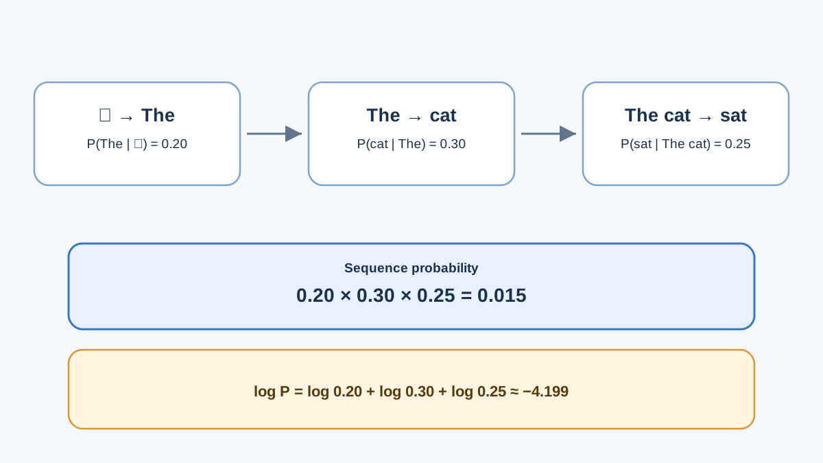
Let's make the product concrete. Take a three-token sequence and assign each step a conditional probability. These are toy values, chosen so the arithmetic is easy to follow.
| Step | Prefix | Chosen token | Conditional probability |
|---|---|---|---|
| 1 | (none) | The | 0.20 |
| 2 | The | cat | 0.30 |
| 3 | The cat | sat | 0.25 |
Multiply:
So under this model, the probability that generation begins with the token sequence The cat sat is 0.015, or about 1.5%.
Read that carefully. It is the probability of this specific three-token prefix under this model. It is not the probability that generation stops here — for that, you would need to include the conditional probability of an end-of-sequence token as a fourth factor. It is not the probability that a cat sat anywhere. It is not a quality score. It is not a truth value. It is a likelihood assigned to a string of tokens.
Now the same number in log space. Take the natural log of each conditional and add:
Exponentiating back gives roughly 0.015, as expected. In practice you would compute and compare the log version, because sums are stable and products are not.
To see how sensitive the product is, change one value. Suppose step 2's conditional drops from 0.30 to 0.10:
One conditional fell by a factor of three, and the sequence probability fell by the same factor. Every step multiplies the whole. That is a property of the arithmetic: longer sequences accumulate more factors, and each factor below one pulls the product down.
Here is the same structure as a left-to-right chain:
[START]
   │  P(The) = 0.20
   ▼
[The]
   │  P(cat | The) = 0.30
   ▼
[The cat]
   │  P(sat | The cat) = 0.25
   ▼
[The cat sat]

P(prefix "The cat sat") = 0.20 × 0.30 × 0.25 = 0.015
Each node is a prefix. Each edge is one conditional. The product is the whole path.
Knowledge check
Check your understanding
Answer this question before you continue.
What the Factorization Does and Does Not Say
Two misreadings cause most of the confusion downstream.
Probability is not certainty. A high-probability sequence is one the model considers likely under its training distribution. It is not verified, guaranteed, or correct. The model can assign high probability to a fluent falsehood and low probability to a correct but unusual phrasing.
Probability is not quality. Fluency, factual accuracy, usefulness, and safety are separate properties. A well-formed sentence and a confidently wrong sentence can carry similar probabilities. The number tells you what the model expects to see, not what you should trust.
There is a third boundary worth stating plainly: the factorization describes how the model scores a sequence, not how it decides to produce one. Decoding choices — greedy selection, sampling, temperature, top-k — sit on top of these probabilities. They change which sequence you get, not what the underlying probability of a given sequence is.
Common mistake: Treating a low-probability output as wrong and a high-probability output as safe. In a retrieval or agent pipeline, the model's likelihood says nothing about whether the retrieved evidence was relevant. Those are different questions with different signals.
Knowledge check
Check your understanding
Answer this question before you continue.
Why This Matters When You Build
Three practical consequences follow from the derivation.
Long outputs compound many conditionals. Every additional token multiplies the running product by another factor. This is why raw sequence probabilities become vanishingly small as sequences grow, and why log-probabilities are the practical currency for scoring, comparing, and thresholding outputs. Raw products underflow; sums do not.
Sequence probability is a narrow signal. It is useful when you want to know how typical a sequence is under a model — for scoring, ranking candidates, or detecting out-of-distribution text. It is not useful as a proxy for correctness, relevance, or safety. A low-probability output is not automatically wrong, and a high-probability output is not automatically trustworthy.
Per-step conditionals are what you can actually inspect. When you want to understand why a particular sequence scored the way it did, look at the individual conditional values, not just the final product. Each one tells you how strongly the model expected that token given its prefix. That is a more granular and more honest signal than the collapsed sequence number.
Tip: My rule is simple. Use sequence probability when the question is "how likely is this text under this model?" Do not use it when the question is "is this text true, relevant, or safe?" Those require different tools — retrieval checks, fact verification, or human review.
Where to Go Next
Compress the whole article into one sentence: a sequence probability is a product of conditional next-token probabilities — exact as a factorization, approximate as a model.
The best way to internalize this is to do it by hand. Pick any short sentence. Write out its prefixes, one token at a time. For each step, estimate the conditional probability yourself — even roughly — and multiply. Watch how fast the product shrinks. Watch how much one weak step drags the whole number down.
Once that feels natural, the next question is how these probabilities become actual text: which token gets picked at each step, and why greedy selection and sampling produce very different outputs from the same distribution. That is where decoding strategies take over.
Knowledge check
Final check
Finish the article by checking the ideas you just learned.
References
Want a more structured LLMOps path?
Use the LLMOps Practical Starter Bundle to connect RAG, evaluation, observability, and production patterns.
Large Language Models Starter Pack
A 12-chapter guide connecting LLM fundamentals with prompting, RAG, agents, tool calling, evaluation, security, and application engineering.
- 227-page Illustrated PDF edition
- 12 guided LLM engineering chapters
- Visual concept diagrams
- Self-assessment quizzes
- Bonus deep-dive sections
- Prompt design, structured output, context windows & RAG pipelines
- Agents, tool calling, prompt injection, evaluation & application lifecycles
Coming soon


