
Measure Agreement Between an LLM Judge and Human Labels
A judge that agrees with humans 90% of the time can still be useless. Here is how to tell the difference.

Key topics
A judge that agrees with humans 90% of the time can still be useless. Here is how to tell the difference.
You built a judge. You labeled a few hundred cases by hand. The judge matches your labels 90% of the time, and someone on the team says: ship it.
Then you look at the label distribution. Ninety percent of your cases carry the same label. A judge that answers that label every single time — no reading, no reasoning, no model — would score the same 90%. Your judge might be doing real work, or it might be a very expensive constant. The percentage cannot tell you which.
That is the problem this article fixes. Agreement is not a property of a judge. It is a property of a measurement protocol: which cases you counted, which labels you used, how you handled the messy ones, and what the label distribution looked like. Change the protocol, and the same verdicts produce a different number.
We will build the protocol from the ground up, derive two agreement statistics from one small table, and work through what each one actually estimates.
What the Agreement Number Is Actually Estimating
Before any formula, fix the measurement target. Four decisions silently move the number, and most teams make them by accident.
The unit of judgment. One case, one criterion, one verdict. If your rubric scores correctness, relevance, and tone, that is three judgments per case, not one. Pooling them into a single agreement number averages away the fact that your judge may be excellent at one criterion and terrible at another.
The reference label. Human labels are not ground truth. They are an operational reference — usually a majority vote across annotators or an adjudicated decision. That distinction matters later, when you compare judge-human agreement against human-human agreement.
Which cases are retained. Dropped cases, refusals, and invalid judge outputs are not neutral. If your judge fails to produce a parseable verdict on the hard cases and you exclude them, you have quietly measured agreement on the easy subset.
Whether verdicts are pooled. Pooling across criteria or across annotators changes what the table means. Decide before you count.
Note: This article assumes you already have a rubric and a human-labeled subset. Rubric design and calibration come first; agreement measurement tells you whether the rubric and the judge are behaving consistently on the cases you kept.
Notation and the Label Table
Start binary. Two labels — positive and negative — one verdict per rater per case. That is enough to expose every trap, and it is the setting most judges actually run in.
Build a contingency table with four cells:
| Human positive | Human negative | |
|---|---|---|
| Judge positive | a | b |
| Judge negative | c | d |
- a: both raters said positive
- b: judge positive, human negative
- c: judge negative, human positive
- d: both said negative
- n = a + b + c + d: total paired cases
The marginals are the row and column totals expressed as rates. The human positive rate is (a + c) / n. The judge positive rate is (a + b) / n. These are called marginal distributions because they live in the margins of the table, and they are about to become the most important numbers in the article.
Four assumptions hold everything together:
- Paired labels. Every case has exactly one human verdict and one judge verdict.
- No missing verdicts. No dropped cases, no refusals, no unparseable outputs.
- Nominal and symmetric labels. Neither rater is designated correct. Agreement is a two-way street.
- One criterion per table. No pooling across rubric dimensions.
Break any of these and the table means something different. Ordinal scales, dropped cases, and pooled criteria all change the interpretation — sometimes dramatically.
Knowledge check
Check your understanding
Answer this question before you continue.
Raw Agreement: The First Number, and Its Blind Spot
Raw agreement is the diagonal mass: the fraction of cases where both raters landed on the same label.
That is it. Compute it by hand on a small table and you will never misread it again.
Suppose you labeled 100 cases. The table comes out:
| Human positive | Human negative | Total | |
|---|---|---|---|
| Judge positive | 20 | 5 | 25 |
| Judge negative | 10 | 65 | 75 |
| Total | 30 | 70 | 100 |
Raw agreement: (20 + 65) / 100 = 0.85.
Eighty-five percent. That sounds strong. Now look at the marginals: humans said positive 30% of the time, the judge said positive 25% of the time. Those are close. The judge is not obviously degenerate.
But here is the blind spot. Imagine a judge that ignores the case entirely and always answers "negative." On this same dataset, it would score 70 / 100 = 0.70 raw agreement while carrying zero information about any individual case. Push the negative rate to 90% and the same constant judge scores 0.90.
This is not a corner case. Imbalanced evaluation sets are the default in most real applications — most outputs are fine, most claims are supported, most answers are relevant. Raw agreement rewards a judge for matching the majority label, and the more imbalanced your set, the more it rewards.
Common mistake: Reporting raw agreement as evidence that a judge works. Raw agreement is a reporting requirement, not a verdict. It tells you how often two raters landed in the same cell. It does not tell you whether the judge is reading the case.
Knowledge check
Check your understanding
Answer this question before you continue.
Chance-Adjusted Agreement: Deriving Cohen's Kappa
The question kappa answers: how much better than random guessing do these two raters agree, given their own label habits?
"Given their own label habits" is the key phrase. If humans say positive 30% of the time and the judge says positive 25% of the time, some agreement is expected by chance alone. Kappa subtracts that expectation out.
Step 1: Expected agreement from the marginals.
If the two raters assigned labels independently at their observed rates, the probability both say positive is the product of the two positive rates. Same for negative. Add them:
On our table: human positive rate = 0.30, judge positive rate = 0.25, human negative rate = 0.70, judge negative rate = 0.75.
Step 2: Observed agreement. Already computed: .
Step 3: Kappa.
The numerator is agreement above chance. The denominator is the room left above chance. Kappa is the fraction of available headroom the raters actually used.
Read the scale: 0 means chance-level agreement, 1 means perfect, negative means worse than chance. Our judge sits at 0.625 — meaningfully above chance, but with a quarter of the headroom still unused.
Compare the two numbers. Raw agreement said 0.85. Kappa said 0.625. Same verdicts, same table, very different stories about how much the judge is actually contributing.
Knowledge check
Check your understanding
Answer this question before you continue.
Why Prevalence Moves the Number
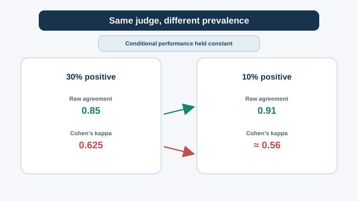
Now hold the judge's behavior fixed and change only the class prevalence. This is the comparison that matters, so it has to be controlled: the judge keeps the same conditional accuracy on positives and negatives, and only the mix of cases shifts.
In the first table, the judge got 20 of 30 positives right (about 0.67) and 65 of 70 negatives right (about 0.93). Keep those rates. Drop the same judge into a dataset where 90% of cases are negative and 10% are positive.
With 100 cases: 10 positives, 90 negatives. At the same rates, the judge catches about 7 of the 10 positives and about 84 of the 90 negatives. Round to whole cases for a clean table:
| Human positive | Human negative | Total | |
|---|---|---|---|
| Judge positive | 7 | 6 | 13 |
| Judge negative | 3 | 84 | 87 |
| Total | 10 | 90 | 100 |
Raw agreement: (7 + 84) / 100 = 0.91. It climbed from 0.85 to 0.91 — and the judge did nothing better. It simply had more easy negatives to match.
Now compute kappa. Human positive rate = 0.10, judge positive rate = 0.13.
Raw agreement rose from 0.85 to 0.91. Kappa fell from 0.625 to about 0.56. Same judge, same conditional skill, different label distribution, opposite signals.
This is the prevalence paradox, and it is not a bug. When one label dominates, chance agreement is high, so the room above chance shrinks. Kappa correctly reports that the judge had less opportunity to demonstrate skill — and that most of its raw agreement came from matching the majority label.
The mirror case is just as instructive. Balanced labels — 50/50 — make chance agreement low, so kappa and raw agreement track closely. If your dataset is balanced and the two numbers diverge sharply, something else is wrong.
Kappa also penalizes marginal mismatch. A judge that assigns the positive label at a very different rate than humans gets punished even when individual verdicts look mostly right. That is a feature: it catches judges that are systematically harsher or more lenient than your annotators, which a raw percentage hides.
Decision rule: Always report raw agreement, kappa, and the label counts together. Never one number alone. The label counts are what let a reader interpret the other two.
Knowledge check
Check your understanding
Answer this question before you continue.
What Agreement Does Not Tell You
Agreement is symmetric. Correctness is not. Two raters can agree with each other and both be wrong against the task requirement. Kappa will happily report 0.9 while your judge and your annotators share the same blind spot.
Human-human agreement is context, not a ceiling. If your annotators only agree with each other 72% of the time, perfect judge agreement is not the target — it is a sign the judge has learned something the humans have not, or that the rubric is ambiguous enough that the judge is exploiting the ambiguity. Report human-human agreement on the same subset as a comparison baseline.
Treat the judge as a classifier. Against the reference labels, compute precision, recall, and the confusion matrix. A single agreement number hides which errors the judge makes. A judge with 0.85 raw agreement that fails on every positive case is a different tool than one with 0.85 that fails evenly.
Aggregate agreement masks subset failures. A judge can score well overall while failing on the subset of cases it could not itself answer. If your judge is also a model that produces answers, its grading ability and its answering ability are correlated — and the aggregate number will not show you where.
When to use agreement checks: calibrating a judge, comparing judge versions, deciding whether a judge is trustworthy enough to automate a decision. When not to: as proof of answer quality, or as a substitute for inspecting failures. Agreement is a consistency check, not a correctness check.
A Reporting Checklist You Can Reuse
Turn the derivation into a protocol you can apply to your own judge.
- Document the unit judged. One case, one criterion, one verdict. State it explicitly.
- State label definitions and whether they are nominal or ordinal.
- Report the case count and label distribution. Both marginals, not just the total.
- Report raw agreement and a chance-adjusted statistic — kappa for two raters, Fleiss' kappa or Krippendorff's alpha for more — with the label counts that produced them.
- Report human-human agreement on the same subset as a baseline.
- Report the confusion matrix or the dominant disagreement pattern, not just the headline number.
- Avoid universal thresholds. "0.6 is good" is not a rule. Whether an agreement level is sufficient depends on task ambiguity, error cost, and how the judge's output will be used.
The 90% judge from the opening was never lying. It was measured badly. Recompute agreement on your own labeled subset, report raw agreement, kappa, and label counts together, and inspect the confusion matrix before you trust the judge with anything that matters.
Once the judge is calibrated, the next move is putting it to work: wiring it into a regression-testing workflow so every system change gets scored against the same fixed cases and the same calibrated grader.
Knowledge check
Final check
Finish the article by checking the ideas you just learned.
References
Want a more structured LLMOps path?
Use the LLMOps Practical Starter Bundle to connect RAG, evaluation, observability, and production patterns.
Large Language Models Starter Pack
A 12-chapter guide connecting LLM fundamentals with prompting, RAG, agents, tool calling, evaluation, security, and application engineering.
- 227-page Illustrated PDF edition
- 12 guided LLM engineering chapters
- Visual concept diagrams
- Self-assessment quizzes
- Bonus deep-dive sections
- Prompt design, structured output, context windows & RAG pipelines
- Agents, tool calling, prompt injection, evaluation & application lifecycles
Coming soon


