
Statistical Uncertainty in LLM Evaluations: Is the Improvement Real?
Version B scores 74%. Version A scored 71%. Same 40 cases, same rubric, and someone in the thread types the sentence that ends the discussion: "So B is…

Key topics
Version B scores 74%. Version A scored 71%. Same 40 cases, same rubric, and someone in the thread types the sentence that ends the discussion: "So B is better, let's ship it."
Maybe. But that three-point gap is doing a lot of unearned work. Before you ship, you need to know whether the gap measures your system or measures your test set's mood that afternoon.
Here is the uncomfortable truth: an eval score is not a property of your system. It is a sample drawn from a noisy process, and the noise has at least two sources. Your job is not to trust the number. Your job is to decide whether the gap between two numbers survives the spread around them.
By the end of this article, you will be able to put a defensible interval around a score, put an interval around the gap between two versions, and apply a decision rule on top of both.
Why a Score Is an Estimate, Not a Verdict
If you have already built a small evaluation set with representative cases and failure labels, you have done the hard part. This article is about what those numbers can and cannot support.
Two sources of wobble stack on top of each other:
- Sampling variability across cases. You did not test every possible input. You tested 40. A different 40 would give a different score.
- Output stochasticity. The same case, run twice, can pass once and fail once. The model is not a function; it is a distribution.
A single number hides both. The same system can score 71% or 78% on two different 40-case draws without anything changing. That is not a bug in your eval. That is the eval working as designed, and you are reading only the point estimate.
The quantity you want is true performance on the task distribution. The quantity you measured is performance on your cases. These are related but not identical, and the gap between them is what statistical uncertainty is about.
Picture a score as a dot sitting inside a band. The dot is what you reported. The band is where the true value plausibly sits. If two dots sit inside each other's bands, you cannot tell them apart.
Notation and Assumptions You Should State Out Loud
Before the math, name the symbols. This is the part most teams skip, and it is where the quiet errors live.
- N: the number of cases in your eval set.
- x_i: the score for case i, usually 0 or 1 for pass/fail.
- p̂ (read "p-hat"): the reported score, computed as the sample mean: p̂ = (1/N) Σ x_i.
- p: the true rate you are trying to estimate. You never observe this directly.
Three assumptions make the math valid. Each one breaks in a specific way.
Assumption 1: Cases are a representative draw from the task distribution. If your 40 cases are hand-picked easy examples, no interval will save you. A confidence interval around a biased estimate is a precise measurement of the wrong thing.
Assumption 2: Per-case outcomes are roughly independent. If ten of your cases use the same source document, the same template, or the same user, they are correlated. Correlated cases shrink your effective sample size below N, which makes your intervals too narrow. You will feel more confident than you should.
Assumption 3: The scoring rule is stable. If a model judge is your grader, grader noise is a second variance source layered on top of sampling noise. You are now measuring two distributions at once.
Common mistake: Treating the interval as a fix for a bad case set. It is not. Intervals quantify sampling error. They do nothing about bias from unrepresentative cases, correlated cases, or an unstable grader.
Knowledge check
Check your understanding
Answer this question before you continue.
The Standard Error of a Score, Derived
Start with one case. The outcome is a Bernoulli draw: pass with probability p, fail with probability 1 − p. Its variance is p(1 − p).
Your reported score is the average of N such draws. When the draws are independent, variances add, and dividing by N scales the variance down by N². So:
Var(p̂) = p(1 − p) / N
The standard error is the square root:
SE = sqrt( p(1 − p) / N )
That is the whole formula. Now watch it work.
Worked example. Suppose p̂ = 0.71 and N = 40.
SE = sqrt( 0.71 × 0.29 / 40 ) = sqrt( 0.2059 / 40 ) = sqrt( 0.00515 ) ≈ 0.072
A rough 95% interval is p̂ ± 1.96 × SE, which gives roughly 0.57 to 0.85. Your "71%" is really "somewhere between 57% and 85%, probably."
Now the same score with N = 400:
SE = sqrt( 0.2059 / 400 ) = sqrt( 0.000515 ) ≈ 0.023
The interval tightens to roughly 0.67 to 0.75. Same score, much sharper claim. That is the sample-size lever, and it is the only one that reliably buys you precision.
One interpretation note: the interval is about the estimate, not about individual cases. It says where the true rate plausibly sits. It does not tell you what any single case will do.
Knowledge check
Check your understanding
Answer this question before you continue.
Where the Textbook Interval Lies to You
The formula above relies on the normal approximation, which assumes the sampling distribution is roughly symmetric and well-behaved. With small N and scores near 0 or 1, it is not. The interval comes out too narrow, noise looks like signal, and teams ship changes that did nothing.
This is not a theoretical worry. Recent work on LLM evaluation has argued directly that Central Limit Theorem–based intervals are inappropriate for small, specialized benchmarks and tend to dramatically underestimate uncertainty in exactly the regime most teams operate in.
A practical boundary: treat normal-approximation intervals as unreliable below a few hundred cases, and be especially suspicious when your score is near the ceiling or floor.
Better alternatives for small-data settings:
- Bootstrap resampling over cases. Resample your N cases with replacement many times, recompute the score each time, and read the interval off the resulting distribution. It makes no symmetry assumption and handles skewed scores gracefully.
- Bayesian or Beta-style intervals. These stay inside [0, 1] and widen honestly when N is small, which is what you want when you have 30 cases and a 90% score.
Note: These methods fix the shape of the interval. They do not fix a biased or unrepresentative case set. If your cases are wrong, a wider interval just tells you more honestly that you do not know.
Repeated Runs: Separating Case Noise From Output Noise
So far we have treated each case as a single pass/fail. But LLMs are stochastic. Run the same case five times and you may get four passes and one fail. That is not a scoring nuisance. That is a reliability finding.
The fix is to run each case k times and record the per-case pass rate instead of a single binary outcome. A case that passes 5 out of 5 is stable. A case that passes 3 out of 5 is flaky, and flaky cases are where your system is actually fragile.
Averaging per-case pass rates across cases gives you a score whose uncertainty now includes both case sampling and run-to-run variation.
Practical guidance:
- 3 to 5 runs per case already reveals whether a case is stable or flaky. More runs buy precision on flaky cases specifically, not uniformly.
- Flag flaky cases separately. A case that flips between pass and fail across runs is a reliability signal, not a rounding error.
- Spend runs where variance is highest. Repeated runs multiply cost and latency. Do not run everything five times if three cases are responsible for most of the wobble.
Tip: If you cannot afford repeated runs on every case, run them on the cases closest to your decision boundary. Those are the ones whose flakiness actually changes your conclusion.
Knowledge check
Check your understanding
Answer this question before you continue.
Comparing Two Versions: Is the Gap Real?
Now the decision you actually face. Version A scored 0.71. Version B scored 0.74. Is the gap real?
Compare the difference, not the two scores in isolation. And when possible, run both versions on the same case set so case difficulty cancels out. This is a paired comparison, and it is far more sensitive than comparing two independent averages.
Deriving the Paired Difference
Let d_i be the difference for case i: the score of B on case i minus the score of A on case i. With binary pass/fail, d_i takes one of three values:
- +1 if B passes and A fails (a win for B)
- −1 if A passes and B fails (a loss for B)
- 0 if both pass or both fail (a tie)
The estimated gap is the average of these per-case differences:
d̄ = (1/N) Σ d_i
The variance of d̄ follows the same logic as before. When cases are independent:
Var(d̄) = Var(d) / N
where Var(d) is the variance of the per-case differences. You can estimate it directly from your data:
Var(d) ≈ (1/(N−1)) Σ (d_i − d̄)²
The standard error of the gap is the square root of Var(d̄). A rough 95% interval is d̄ ± 1.96 × SE(d̄).
The key insight: you are computing uncertainty on the differences, not on the two scores separately. This is what makes pairing powerful. If B wins on the hard cases and ties on the easy ones, the per-case differences capture that structure. Comparing two independent score intervals throws it away.
Worked Example: The 12-9-19 Split
Suppose B beats A on 12 cases, loses on 9, and ties on 19. That is N = 40.
The gap is d̄ = (12 − 9) / 40 = 3/40 = 0.075, or 7.5 percentage points.
Now compute the variance of the per-case differences. With 12 wins (+1), 9 losses (−1), and 19 ties (0):
Σ (d_i − d̄)² = 12(1 − 0.075)² + 9(−1 − 0.075)² + 19(0 − 0.075)² = 12(0.856) + 9(1.156) + 19(0.0056) = 10.27 + 10.40 + 0.11 = 20.78
Var(d) ≈ 20.78 / 39 ≈ 0.533
SE(d̄) = sqrt(0.533 / 40) = sqrt(0.0133) ≈ 0.115
The 95% interval around the gap is roughly 0.075 ± 1.96 × 0.115, which spans from about −0.15 to +0.30. That interval comfortably includes zero. The "7.5-point improvement" is not distinguishable from noise at this sample size.
Notice what happened: the gap looked bigger than the original 3-point claim, but the uncertainty around it is also large. The honest answer is not yet demonstrated.
Knowledge check
Check your understanding
Answer this question before you continue.
Worked Example: Larger N
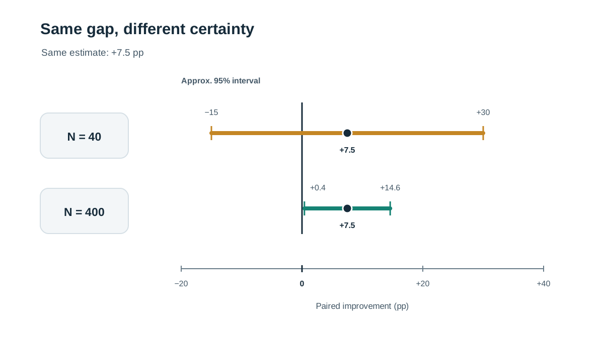
Now suppose the same 7.5-point gap on 400 cases, with the same win/loss/tie proportions scaled up: 120 wins, 90 losses, 190 ties.
d̄ = (120 − 90) / 400 = 0.075
Σ (d_i − d̄)² = 120(0.925)² + 90(1.075)² + 190(0.075)² = 120(0.856) + 90(1.156) + 190(0.0056) = 102.7 + 104.0 + 1.1 = 207.8
Var(d) ≈ 207.8 / 399 ≈ 0.521
SE(d̄) = sqrt(0.521 / 400) = sqrt(0.0013) ≈ 0.036
The 95% interval is roughly 0.075 ± 0.071, or about 0.004 to 0.146. That interval excludes zero. Now you have a defensible improvement claim.
Connecting Repeated Runs to the Paired Comparison
If your cases are stochastic, you are not working with a single binary outcome per case. You are working with a per-case pass rate. The paired difference becomes:
d_i = (pass rate of B on case i) − (pass rate of A on case i)
This d_i is now a continuous value between −1 and +1, not just −1, 0, or +1. The same formulas apply: average the per-case differences, compute their variance, and derive the standard error. The only change is that ties become "similar pass rates" rather than exact matches.
This is the bridge between the repeated-runs section and the comparison section. Run each case k times, compute per-case pass rates for both versions, take the difference per case, and then apply the paired-difference math.
Common mistake: Comparing two independent score intervals and declaring "no overlap means real improvement." Overlap between separate intervals is not the right test. The right test is whether the interval around the paired gap excludes zero.
Power, Effect Size, and What "Meaningful" Means
Statistical significance answers one question: could this be noise? It does not answer whether the improvement matters to users. A tiny, real improvement can be worthless.
Set a minimum meaningful effect before you run the comparison. Then ask whether your case count can even detect it. If it cannot, your eval is underpowered by design, and no amount of staring at the result will fix that.
Rough intuition: detecting smaller effects requires quadratically more cases. Halving the effect you want to catch roughly quadruples the cases you need. This is why "just add a few more cases" rarely rescues an underpowered eval.
Asymmetry matters too. For safety or risk checks, a missed regression is often costlier than a false alarm. That argues for wider margins and more cases on the risky slice, not uniform coverage.
Common mistake: Treating statistical significance as the goal. It is a gate, not a finish line. Report the effect size and its interval together, and state the threshold you would act on.
Common Mistakes That Manufacture Fake Improvements
A compact checklist you can run against your own eval before trusting a result:
| Mistake | What it does to your conclusion |
|---|---|
| Reusing the same cases to tune prompts, then reporting improvement on them | The score is fitted to the test set. Improvement is partly memorization. |
| Reporting the best of several runs instead of the average | Selects for luck. Inflates the score and hides variance. |
| Ignoring correlated cases | Effective sample size is far smaller than N. Intervals are too narrow. |
| Treating a model-judge score as ground truth | Grader noise and bias (e.g., toward longer answers) become invisible. |
| Changing the case set between versions | The two scores are no longer comparable. |
| Comparing two independent averages instead of paired cases | Throws away the sensitivity that pairing gives you. |
A Practical Reporting Habit
Theory is only useful if it changes what you write down. Here is the format I would adopt immediately.
For every version comparison, report five things:
- Case count (N) and run count per case (k).
- Score for each version.
- Uncertainty interval around each score.
- The paired gap and its interval.
- The minimum meaningful effect you defined before running the comparison.
Then add two lines of judgment:
- Flag any cases that were unstable across runs.
- State whether the gap interval excludes zero and clears your threshold.
Keep the case set frozen across the comparison, and record when it changes. This format is what makes a regression-testing workflow trustworthy rather than ceremonial.
The Decision Rule
Before you claim an improvement, put an interval around the paired gap. Check two things: does it exclude zero, and does it clear your minimum meaningful effect?
If yes, ship with evidence. If no, the honest next move is more cases or more runs on the slice that matters, not a louder claim.
The next practical step is to wire this uncertainty layer into your evaluation harness so every version comparison reports a paired gap with its band, automatically. That is the difference between an eval that produces numbers and an eval that produces decisions.
Knowledge check
Final check
Finish the article by checking the ideas you just learned.
References
Want a more structured LLMOps path?
Use the LLMOps Practical Starter Bundle to connect RAG, evaluation, observability, and production patterns.
Large Language Models Starter Pack
A 12-chapter guide connecting LLM fundamentals with prompting, RAG, agents, tool calling, evaluation, security, and application engineering.
- 227-page Illustrated PDF edition
- 12 guided LLM engineering chapters
- Visual concept diagrams
- Self-assessment quizzes
- Bonus deep-dive sections
- Prompt design, structured output, context windows & RAG pipelines
- Agents, tool calling, prompt injection, evaluation & application lifecycles
Coming soon


